Difference between revisions of "ISSS608 2017-18 T3 Assign Vaishnavi Praveen Agarwal DataPrep"
| (102 intermediate revisions by the same user not shown) | |||
| Line 33: | Line 33: | ||
|} | |} | ||
| − | + | ||
| − | <div style="margin:0px; padding: 2px | + | =Data Description= |
| + | <div style="margin:0px; padding: 2px; font-family: Arial; border-radius: 1px; text-align:left"> | ||
{| class="wikitable" style="background-color:#FFFFFF;" width="100%" | {| class="wikitable" style="background-color:#FFFFFF;" width="100%" | ||
|- | |- | ||
| − | | | + | |style="text-align:center"| |
| − | <b> | + | ; |
| + | <b>File Name</b> | ||
| + | |style="text-align:center"| | ||
| + | <b>Variables</b> | ||
| + | |||
| + | |- | ||
| + | | | ||
| + | <b>Boonsong Lekagul waterways readings (.csv file)</b> | ||
|| | || | ||
| − | |||
| − | |||
| − | |||
| + | The given data file has reading of 106 chemicals at 10 different locations from 1998 - 2016. | ||
| + | |||
| + | <b>i. id</b> (numeric , unique) | ||
| + | <br><b>ii. value</b> (numeric) | ||
| + | <br><b>iii. location</b> (string) | ||
| + | <br><b>iv. sample date</b> (string) | ||
| + | <br><b>v. measure</b> (string) | ||
| + | |||
|- | |- | ||
| | | | ||
| − | + | <b>chemical units of measure (.csv file)</b> | |
| − | |||
| − | <b> | ||
|| | || | ||
| − | |||
| − | |||
| − | + | The given data file has the unit of each measure (106 measures) in which the readings were taken. | |
| − | |||
| − | |||
| − | |||
| − | |||
| − | |||
| − | |||
| + | <b>i. measure</b> (string, unique) | ||
| + | <br><b>ii. unit</b> (string) | ||
| − | |||
| − | |||
| − | |||
| − | |||
| − | |||
| − | |||
|- | |- | ||
| − | + | | | |
| − | + | <b>Waterways Final (.jpg file)</b> | |
| − | |||
| − | |||
| − | <b> | ||
|| | || | ||
| − | |||
| − | |||
| − | |||
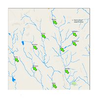
| + | The Waterways Final is a map image that shows the location of dumping site and the waterways. | ||
| + | <span style=text-align:center;">[[Image:Waterways Final.jpg|200px|thumb|left]]</span> | ||
| − | + | |} | |
| − | + | </div> | |
| − | |||
| − | |||
| − | |||
| − | |||
| − | |||
| − | |||
| − | |||
| + | =Data Preparation= | ||
| + | ===1. Grouping Measures=== | ||
| − | + | There are a total of 106 measures given in the data file, and it is difficult to view all the measures at a glance. In order to make the visualization simple I have grouped the measure based on their Chemical Composition and Behavior. | |
| − | |||
| − | |||
| + | - A new column was added in the file <b>chemical units of measure.csv</b> | ||
| + | <br>- Name the column as <b>groups</b> | ||
| + | <br>- Chemical properties of each measure was studied and they were divided in <b>12 groups</b>. | ||
| + | <br>- Manually assigned the relevant group to each measure. | ||
| − | <b> | + | <b>The 12 groups formed are:</b> |
| − | |||
| − | |||
| − | |||
| − | |||
| − | |||
| − | |||
| − | |||
| + | <div style="margin:0px; padding: 2px; font-family: Arial; border-radius: 1px; text-align:left"> | ||
| + | {| class="wikitable" style="background-color:#FFFFFF;" width="100%" | ||
| + | |- | ||
| + | |style="text-align:center"| | ||
| + | ; | ||
| + | <b>Groups</b> | ||
| + | |style="text-align:center"| | ||
| + | <b>Measures</b> | ||
| − | <b> | + | |- |
| − | + | | | |
| − | + | <b>Field measurements</b> | |
| + | || | ||
| + | Anionic active surfactants, Fecal coliforms, Fecal streptococci, Total coliforms, Total extractable matter, Total hardness | ||
| + | |||
| + | |- | ||
| + | | | ||
| + | <b>Heavy metals</b> | ||
| + | || | ||
| − | + | Arsenic, Cadmium, Chromium, Copper, Iron, Lead, Manganese, Mercury, Nickel, Zinc | |
| − | |||
| − | |||
| − | |||
|- | |- | ||
| | | | ||
| − | + | <b>Hydrocarbon</b> | |
|| | || | ||
| − | <b> | + | |
| + | Acenaphthene, Acenaphthylene, Anthracene, Benzo(a)anthracene, Benzo(a)pyrene, Benzo(b)fluoranthene, Benzo(g,h,i)perylene, Benzo(k)fluoranthene, Chrysene, Fluoranthene, Fluorene, Indeno(1,2,3-c,d)pyrene, Naphthalene, PAHs, Pentachlorobenzene, Petroleum hydrocarbons, Phenanthrene, Pyrene, Tetrachloromethane | ||
| + | |||
| + | |- | ||
| + | | | ||
| + | <b>Insecticides, Pesticides and Herbicides</b> | ||
|| | || | ||
| − | |||
| − | <b> | + | Alachlor, Aldrin, Atrazine, Endosulfan (alpha), Endosulfan (beta), gamma-Hexachlorocyclohexane, Isodrin, Methoxychlor, Metolachlor, p,p-DDD, p,p-DDE, p,p-DDT, Simazine, Trifluralin |
| − | + | ||
| − | + | |- | |
| + | | | ||
| + | <b>Metal</b> | ||
| + | || | ||
| + | Aluminium, Barium, Berilium, Boron, Calcium, Cesium, Magnesium, Potassium, Selenium, Sodium | ||
| − | <b> | + | |- |
| − | + | | | |
| − | + | <b>Mineral and Nutrients</b> | |
| − | + | || | |
| − | |||
| − | |||
| + | Dissolved silicates, Orthophosphate-phosphorus, Silica (SiO2), Total dissolved phosphorus, Total nitrogen, Total phosphorus | ||
| − | <b> | + | |- |
| − | + | | | |
| − | + | <b>Nitrogen</b> | |
| + | || | ||
| + | Inorganic nitrogen, Organic nitrogen, Total organic carbon | ||
| − | |||
| − | |||
| − | |||
|- | |- | ||
| | | | ||
| − | + | <b>Organic</b> | |
| − | |||
| − | <b> | ||
|| | || | ||
| − | |||
| − | + | alpha-Hexachlorocyclohexane, AOX, beta-Hexaxchlorocyclohexane, Dieldrin, Endrin, Heptachlor, Heptachloroepoxide, Hexachlorobenzene, PCB 101, PCB 118, PCB 138, PCB 153, PCB 180, PCB 28, PCB 52 | |
| − | |||
| − | |||
| + | |- | ||
| + | | | ||
| + | <b>Others</b> | ||
| + | || | ||
| − | + | 1,2,3-Trichlorobenzene, 1,2,4-Trichlorobenzene, AGOC-3A, Macrozoobenthos, Methylosmoline | |
| − | |||
| − | |||
| + | |- | ||
| + | | | ||
| + | <b>Oxygen</b> | ||
| + | || | ||
| − | + | Biochemical Oxygen, Chemical Oxygen Demand (Cr), Chemical Oxygen Demand (Mn), Dissolved organic carbon, Dissolved oxygen, Oxygen saturation | |
| − | |||
| − | |||
| + | |- | ||
| + | | | ||
| + | <b>Salt</b> | ||
| + | || | ||
| − | + | Ammonium, Bicarbonates, Carbonates, Chlorides, Chlorodinine, Cyanides, Nitrates, Nitrites, Sulfides, Sulphates, Total dissolved salts | |
| − | |||
| − | |||
|- | |- | ||
| | | | ||
| − | + | <b>Water temperature</b> | |
|| | || | ||
| − | |||
| − | |||
| − | |||
| − | |||
| − | |||
| − | |||
| − | |||
| + | Water temperature | ||
| + | |||
| + | |} | ||
| + | </div> | ||
| − | + | ===2. Coordinate Plotting=== | |
| − | |||
| − | |||
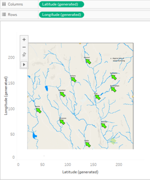
| + | Waterways Final is a Map image provided in the data, but the data files does not contain Latitude and Longitude for the Places shown on the Map. Therefore, to use the Map as an interactive sheet, I will create the Latitude and Longitude manually in the following way: | ||
| − | <b> | + | <div style="margin:0px; padding: 2px; font-family: Arial; border-radius: 1px; text-align:left"> |
| − | + | {| class="wikitable" style="background-color:#FFFFFF;" width="100%" | |
| − | + | |- | |
| + | |style="text-align:center"| | ||
| + | ; | ||
| + | <b>Steps</b> | ||
| + | |style="text-align:center"| | ||
| + | <b>Image</b> | ||
| + | |- | ||
| + | | | ||
| + | <b>Adding Data and Background Image for Map</b> | ||
| − | + | *Open Boonsong Lekagul waterways readings (.csv file) in Tableau, right click on Location Dimension, click on Geographic Role and select ZIP Code / Postcode. This will generate Latitude and Longitude in Measures. Add the generated fields to Columns and Rows respectively. | |
| − | * | + | *Go to Map options and click on Background Images. In the dialogue box, browse the Waterways Final (.jpg file). In the X Field set Right value to 249 and in the Y Field set the Top value to 249. Go to options and select Always show entire image option and Apply. |
| − | + | ||
| + | || | ||
| + | <span style=text-align:center;">[[Image:Vaishnavi_1.png|300px|thumb|center]]</span> | ||
|- | |- | ||
| | | | ||
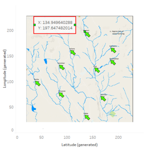
| − | + | <b>Annotate Point to generate Coordinates</b> | |
| + | |||
| + | *Create a new excel file Locations, add a column named Location and manually enter the places. Add other two column named X and Y. | ||
| + | *Right click on the tip of the arrow on map, click on Annotate and select Point. | ||
| + | *In the dialog box, insert fields Latitude(generated) and Longitude(generated). | ||
| + | *Manually copy paste the annotated values in the Location.xlsx file, X and Y columns. | ||
| + | *Do this for all the locations. | ||
| + | |||
|| | || | ||
| − | < | + | <span style=text-align:center;">[[Image:Vaishnavi_2.png|300px|thumb|center]]</span> |
| − | || | ||
| − | |||
| − | |||
| − | |||
| − | |||
| + | |} | ||
| + | </div> | ||
| − | + | ===3. Combining Files=== | |
| − | |||
| − | |||
| − | |||
| + | After cleaning and preparing the data, we have total 3 files: <b>Boonsong Lekagul waterways readings (.csv file)</b>, <b>chemical units of measure (.csv file)</b> and <b>Location (.xlsx file)</b>. We will combine these file using the common columns as Join clause and then do the Visualization. | ||
| + | |||
| + | <div style="margin:0px; padding: 2px; font-family: Arial; border-radius: 1px; text-align:left"> | ||
| + | {| class="wikitable" style="background-color:#FFFFFF;" width="100%" | ||
| + | |- | ||
| + | |style="text-align:center"| | ||
| + | ; | ||
| + | <b>Steps</b> | ||
| + | |style="text-align:center"| | ||
| + | <b>Image</b> | ||
| − | |||
| − | |||
| − | |||
| − | |||
| − | |||
| − | |||
| − | |||
| − | |||
| − | |||
| − | |||
| − | |||
|- | |- | ||
| | | | ||
| − | + | <b>Combining Boonsong Lekagul waterways readings (.csv file) and chemical units of measure (.csv file)</b> | |
| + | |||
|| | || | ||
| − | <b> | + | *Open the Data Source, add a new Text File <b>Boonsong Lekagul waterways readings (.csv file)</b>. |
| + | *Again click on Add in Connections, click on Text File and add <b>chemical units of measure (.csv file)</b>. | ||
| + | *Click on Join and select <b>Left Join</b>. | ||
| + | <span style=text-align:center;">[[Image:Vaishnavi_3.png|550px|thumb|center]]</span> | ||
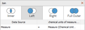
| + | *Use <b>Measure</b> as the Join clause between the two files. | ||
| + | <span style=text-align:center;">[[Image:Vaishnavi_4.png|300px|thumb|center]]</span> | ||
| + | |||
| + | |||
| + | |- | ||
| + | | | ||
| + | <b>Combining Boonsong Lekagul waterways readings (.csv file) and Location (.xlsx file)</b> | ||
| + | |||
|| | || | ||
| − | <b> | + | *Open the Data Source, add a new Microsoft Excel File <b>Location (.xlsx file)</b>. |
| − | * | + | *Click on Join and select <b>Left Join</b>. |
| − | * | + | <span style=text-align:center;">[[Image:Vaishnavi_5.png|400px|thumb|center]]</span> |
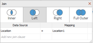
| − | + | *Use <b>Location</b> as the Join clause between the two files. | |
| − | + | <span style=text-align:center;">[[Image:Vaishnavi_6.png|300px|thumb|center]]</span> | |
| − | |||
| − | |||
| − | |||
| − | |||
| − | |||
| − | |||
| − | |||
| − | |||
| − | |||
|} | |} | ||
</div> | </div> | ||
| + | |||
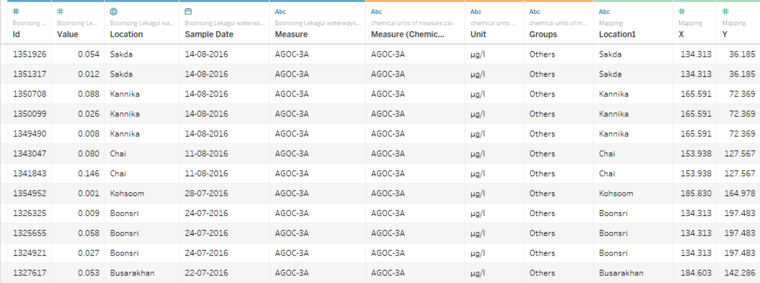
| + | ===4. Final Dataset=== | ||
| + | |||
| + | |||
| + | |||
| + | <span style=text-align:center;">[[Image:Vaishnavi_7.png|1100px|thumb|left]]</span> | ||
Latest revision as of 11:44, 8 July 2018
|
|
|
|
|
|
|
Contents
Data Description
|
File Name |
Variables |
|
Boonsong Lekagul waterways readings (.csv file) |
The given data file has reading of 106 chemicals at 10 different locations from 1998 - 2016. i. id (numeric , unique)
|
|
chemical units of measure (.csv file) |
The given data file has the unit of each measure (106 measures) in which the readings were taken. i. measure (string, unique)
|
|
Waterways Final (.jpg file) |
The Waterways Final is a map image that shows the location of dumping site and the waterways. |
Data Preparation
1. Grouping Measures
There are a total of 106 measures given in the data file, and it is difficult to view all the measures at a glance. In order to make the visualization simple I have grouped the measure based on their Chemical Composition and Behavior.
- A new column was added in the file chemical units of measure.csv
- Name the column as groups
- Chemical properties of each measure was studied and they were divided in 12 groups.
- Manually assigned the relevant group to each measure.
The 12 groups formed are:
|
Groups |
Measures |
|
Field measurements |
Anionic active surfactants, Fecal coliforms, Fecal streptococci, Total coliforms, Total extractable matter, Total hardness |
|
Heavy metals |
Arsenic, Cadmium, Chromium, Copper, Iron, Lead, Manganese, Mercury, Nickel, Zinc |
|
Hydrocarbon |
Acenaphthene, Acenaphthylene, Anthracene, Benzo(a)anthracene, Benzo(a)pyrene, Benzo(b)fluoranthene, Benzo(g,h,i)perylene, Benzo(k)fluoranthene, Chrysene, Fluoranthene, Fluorene, Indeno(1,2,3-c,d)pyrene, Naphthalene, PAHs, Pentachlorobenzene, Petroleum hydrocarbons, Phenanthrene, Pyrene, Tetrachloromethane |
|
Insecticides, Pesticides and Herbicides |
Alachlor, Aldrin, Atrazine, Endosulfan (alpha), Endosulfan (beta), gamma-Hexachlorocyclohexane, Isodrin, Methoxychlor, Metolachlor, p,p-DDD, p,p-DDE, p,p-DDT, Simazine, Trifluralin |
|
Metal |
Aluminium, Barium, Berilium, Boron, Calcium, Cesium, Magnesium, Potassium, Selenium, Sodium |
|
Mineral and Nutrients |
Dissolved silicates, Orthophosphate-phosphorus, Silica (SiO2), Total dissolved phosphorus, Total nitrogen, Total phosphorus |
|
Nitrogen |
Inorganic nitrogen, Organic nitrogen, Total organic carbon |
|
Organic |
alpha-Hexachlorocyclohexane, AOX, beta-Hexaxchlorocyclohexane, Dieldrin, Endrin, Heptachlor, Heptachloroepoxide, Hexachlorobenzene, PCB 101, PCB 118, PCB 138, PCB 153, PCB 180, PCB 28, PCB 52 |
|
Others |
1,2,3-Trichlorobenzene, 1,2,4-Trichlorobenzene, AGOC-3A, Macrozoobenthos, Methylosmoline |
|
Oxygen |
Biochemical Oxygen, Chemical Oxygen Demand (Cr), Chemical Oxygen Demand (Mn), Dissolved organic carbon, Dissolved oxygen, Oxygen saturation |
|
Salt |
Ammonium, Bicarbonates, Carbonates, Chlorides, Chlorodinine, Cyanides, Nitrates, Nitrites, Sulfides, Sulphates, Total dissolved salts |
|
Water temperature |
Water temperature |
2. Coordinate Plotting
Waterways Final is a Map image provided in the data, but the data files does not contain Latitude and Longitude for the Places shown on the Map. Therefore, to use the Map as an interactive sheet, I will create the Latitude and Longitude manually in the following way:
|
Steps |
Image |
|
Adding Data and Background Image for Map
|
|
|
Annotate Point to generate Coordinates
|
3. Combining Files
After cleaning and preparing the data, we have total 3 files: Boonsong Lekagul waterways readings (.csv file), chemical units of measure (.csv file) and Location (.xlsx file). We will combine these file using the common columns as Join clause and then do the Visualization.
|
Steps |
Image |
|
Combining Boonsong Lekagul waterways readings (.csv file) and chemical units of measure (.csv file) |
|
|
Combining Boonsong Lekagul waterways readings (.csv file) and Location (.xlsx file) |
|

