ISSS608 2017-18 T3 Assign Harisingh Data Preparation
Contents
Methodology
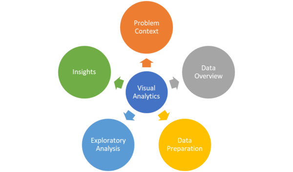
Regardless of the problem complexity, most of the analytics questions in a given business context can be answered using standard approach. The approach, I have considered to analyze chemical contamination around Boonsong Lekagul Wildlife Preserve, is no different whereby I attempt to solve the problem in following sequence:
- Understand the problem context
- Understand the structure of data
- Prepare data for required analysis
- Perform exploratory analysis to understand trend in chemical readings
- Draw meaningful insights useful for hydrology department to further investigate
As depicted in above diagram, Interactive visualization is the core of our solution approach. By nature, analytics solutions are not sequential but often executed in iterative fashion where analysts move back and forth among different stages of analysis.
To garner a holistic idea of chemical contamination, we would attempt to solve the problem using different visualization techniques such as time-series analysis of observed readings. In the process, we also attempt to build useful dashboards to be used by investigators for further analysis.
Tools Used
- Tableau
- R
Problem Context
From the problem statement, I understand that Kasios Furniture Company was accused, by previous year mini challenge participants, of dumping industrial wastes implicating severe environmental damage to the Boonsong Lekagul Wildlife Preserve and its habitats. The approximate location of the dumping site is indicated in given location map, around Kohsoom and Boonsri locations. the dumping of toxic waste seems to have occurred in recent past.
Furthermore, Methylosmolene was identified to be primary toxic manufacturing chemical in the suspected dumping. Since the water sensors data includes several years of observed readings for different chemicals, I plan to take a holistic approach towards this problem and analyze interesting trends in different chemicals.
Data Overview
We are provided with 3 different data sources described as below. The location map is used for Geo-spatial analysis of chemical contamination.
Readings Data
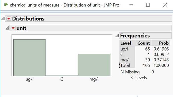
Units Data
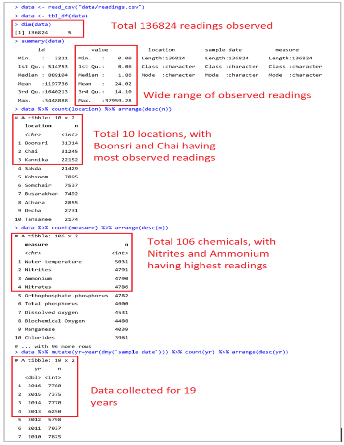
I have used R (tidyverse package) to gather initial understanding of given data. The summary data obtained using R helps us to learn the following:
- A total of 136824 readings were registered, between 1998 and 2016.
- For certain chemicals, readings were observed as high as 37959.
- The number of readings differ widely in different locations.
- Only 21 chemicals, out of 106, have readings for all years. This data would help us to understand the overall trend for such chemicals.
Data Preparation
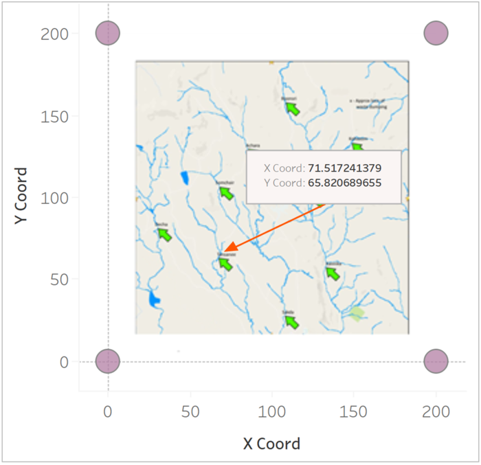
To perform Geo-spatial analysis of chemical contamination, we need to obtain Geo-location for all locations. I have used the point annotation functionality of Tableau to obtain the X-Y coordinates for individual locations. The location map is fitted into scatter plot with approximate range of X-Y axes obtained from MC1 data.
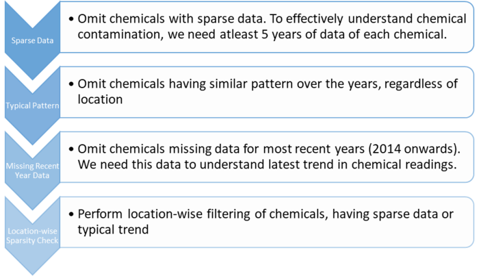
During the data overview section, I observed that not all chemicals have readings registered for all years. To effectively deal with data sparsity issues, I have used multi-level filtering approach where I analyze trend for each chemical, carefully omitting the ones which have insufficient data for analysis or haven’t shown any meaningful trend over the years.
Overall Sparsity Check
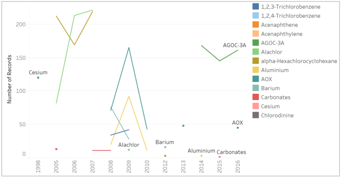
The below line chart highlights those chemicals, which have very sparse data. With data for only 2-3 years, it would be hard for us to clearly understand the overall pattern, so I have filtered out (using filtering at data source level in Tableau) such chemicals, approximately 65, from further analysis.
Typical Pattern Analysis
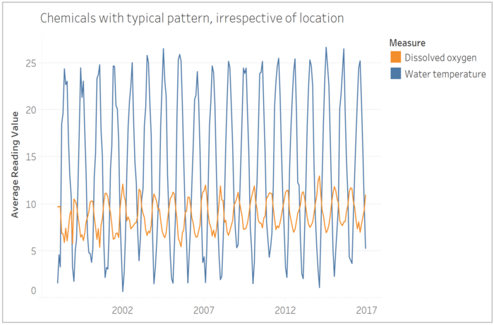
It is evident from below line chart that water temperature and dissolved oxygen have shown very consistent pattern in readings across years in all locations. Since we are more interested into finding unconventional pattern in form of chemical contamination, such chemicals can also be discarded for further analysis.
Additional chemicals which show similar behaviour are oxygen saturation, iron, gamma-Hexachlorocyclohexane, dissolved silicates, dissolved oxygen, calcium, biochemical oxygen, bicarbonates, anionic active surfactants.
Location-wise Sparsity Check
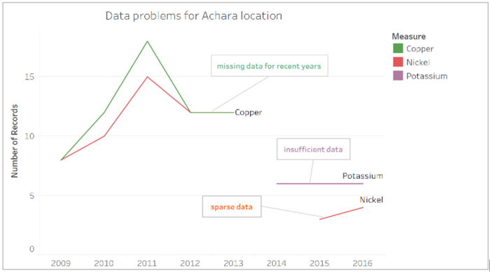
To further drill down into data problems, we zoom into each location data. Interestingly, I encountered similar issues at location level summarized in below line chart. For example, Copper doesn’t have data for recent years in Achara.
Following the multi-level filtering approach, we are left with chemicals, which have readings either for all years or at least in recent years.

