Difference between revisions of "SMT201 AY2019-20G2 Ex2 JerryTohvan"
(Created page with "== Part 1: Thematic Mapping == The thematic mapping developed uses these following data and applied techniques: <br> {| class="wikitable" |- ! Data !! Visualisation & Process...") |
|||
| (19 intermediate revisions by the same user not shown) | |||
| Line 1: | Line 1: | ||
| − | == Part 1: | + | == Part 1: Study Area Map Components == |
| − | |||
| − | |||
| − | |||
| − | |||
| − | |||
| − | |||
| − | + | [[File:Overview map.jpg|700px|center]] | |
| − | |||
| − | [[File: | ||
<p class=MsoNormal align=center style='text-align:center;line-height:normal'><span | <p class=MsoNormal align=center style='text-align:center;line-height:normal'><span | ||
lang=EN-GB style='font-size:8.0pt;font-family:"Times New Roman",serif; | lang=EN-GB style='font-size:8.0pt;font-family:"Times New Roman",serif; | ||
| Line 17: | Line 9: | ||
lang=EN-GB style='font-size:8.0pt;font-family:"Times New Roman",serif; | lang=EN-GB style='font-size:8.0pt;font-family:"Times New Roman",serif; | ||
mso-fareast-font-family:"Times New Roman";font-variant:small-caps;color:white'><span | mso-fareast-font-family:"Times New Roman";font-variant:small-caps;color:white'><span | ||
| − | style='color:windowtext'> | + | style='color:windowtext'>Study Area Map Components</span></span></p> |
| − | </span></span></p> | + | <br><br> |
| + | Firstly, the above summarises an overview of the study area and its map components we want to consider in this suitability land analysis for the Communicable Disease Quarantine Centre in Bukit Gombak. | ||
| + | <br><br> | ||
| + | [[File:Map Target Roads.jpg|600px|center]] | ||
| + | <p class=MsoNormal align=center style='text-align:center;line-height:normal'><span | ||
| + | lang=EN-GB style='font-size:8.0pt;font-family:"Times New Roman",serif; | ||
| + | mso-fareast-font-family:"Times New Roman";font-variant:small-caps;color:white'><span | ||
| + | style='color:windowtext'>FIGURE II</span></span></p> | ||
| + | <p class=MsoNormal align=center style='text-align:center;line-height:normal'><span | ||
| + | lang=EN-GB style='font-size:8.0pt;font-family:"Times New Roman",serif; | ||
| + | mso-fareast-font-family:"Times New Roman";font-variant:small-caps;color:white'><span | ||
| + | style='color:windowtext'>Target Road Map</span></span></p> | ||
| + | <br> | ||
| + | <br> | ||
| + | Figure II shows Bukit Gombak's Road Network that will be accounted in as an Accesibility factor in weighing the location suitability. | ||
<br> | <br> | ||
| − | |||
| − | |||
| − | |||
| − | |||
| − | |||
| − | |||
| − | |||
<br> | <br> | ||
| − | |||
| − | |||
| − | |||
| − | + | [[File:Map Buildings.jpg|600px|center]] | |
| − | [[File: | ||
<p class=MsoNormal align=center style='text-align:center;line-height:normal'><span | <p class=MsoNormal align=center style='text-align:center;line-height:normal'><span | ||
lang=EN-GB style='font-size:8.0pt;font-family:"Times New Roman",serif; | lang=EN-GB style='font-size:8.0pt;font-family:"Times New Roman",serif; | ||
mso-fareast-font-family:"Times New Roman";font-variant:small-caps;color:white'><span | mso-fareast-font-family:"Times New Roman";font-variant:small-caps;color:white'><span | ||
| − | style='color:windowtext'>FIGURE | + | style='color:windowtext'>FIGURE III</span></span></p> |
<p class=MsoNormal align=center style='text-align:center;line-height:normal'><span | <p class=MsoNormal align=center style='text-align:center;line-height:normal'><span | ||
lang=EN-GB style='font-size:8.0pt;font-family:"Times New Roman",serif; | lang=EN-GB style='font-size:8.0pt;font-family:"Times New Roman",serif; | ||
mso-fareast-font-family:"Times New Roman";font-variant:small-caps;color:white'><span | mso-fareast-font-family:"Times New Roman";font-variant:small-caps;color:white'><span | ||
| − | style='color:windowtext'> | + | style='color:windowtext'>Target Building Map</span></span></p> |
| − | </span></span></p> | + | <br> |
| − | <br><br> | + | <br> |
| − | + | Figure III shows Bukit Gombak's Buildings that will be accounted in as an Health Risk factor in weighing the location suitability. We want the Disease Quarantine Centre to be further away from residential in order to ensure safe-zone. Health Risk factor will be prioritised as for the very fact that a Quarantine Centre exists, to ensure no further disease spreading. Bukit Gombak has mostly residential areas in its'subzone. | |
| + | <br> | ||
| + | <br> | ||
| − | + | [[File:Map Natural Features.jpg|600px|center]] | |
| − | |||
| − | |||
| − | |||
| − | |||
| − | [[File: | ||
<p class=MsoNormal align=center style='text-align:center;line-height:normal'><span | <p class=MsoNormal align=center style='text-align:center;line-height:normal'><span | ||
lang=EN-GB style='font-size:8.0pt;font-family:"Times New Roman",serif; | lang=EN-GB style='font-size:8.0pt;font-family:"Times New Roman",serif; | ||
| Line 60: | Line 52: | ||
lang=EN-GB style='font-size:8.0pt;font-family:"Times New Roman",serif; | lang=EN-GB style='font-size:8.0pt;font-family:"Times New Roman",serif; | ||
mso-fareast-font-family:"Times New Roman";font-variant:small-caps;color:white'><span | mso-fareast-font-family:"Times New Roman";font-variant:small-caps;color:white'><span | ||
| − | style='color:windowtext'> | + | style='color:windowtext'>Target Natural Features Map</span></span></p> |
| − | </span></span></p> | ||
| − | |||
| − | |||
| − | |||
| − | |||
| − | |||
| − | |||
| − | |||
| − | |||
| − | |||
| − | |||
| − | |||
<br> | <br> | ||
| − | [[File: | + | [[File:Buffered Merge Waterway.jpg|500px|center]] |
<p class=MsoNormal align=center style='text-align:center;line-height:normal'><span | <p class=MsoNormal align=center style='text-align:center;line-height:normal'><span | ||
lang=EN-GB style='font-size:8.0pt;font-family:"Times New Roman",serif; | lang=EN-GB style='font-size:8.0pt;font-family:"Times New Roman",serif; | ||
| Line 82: | Line 62: | ||
lang=EN-GB style='font-size:8.0pt;font-family:"Times New Roman",serif; | lang=EN-GB style='font-size:8.0pt;font-family:"Times New Roman",serif; | ||
mso-fareast-font-family:"Times New Roman";font-variant:small-caps;color:white'><span | mso-fareast-font-family:"Times New Roman";font-variant:small-caps;color:white'><span | ||
| − | style='color:windowtext'> | + | style='color:windowtext'>Incomplete Waterway Target Inclusion. Applying buffering and merging of polygons in QGIS.</span></span></p> |
| + | |||
<br> | <br> | ||
| − | |||
<br> | <br> | ||
| − | [[File: | + | Figure IV shows Bukit Gombak's Natural Features that will be accounted in as an Natural Conservation factor in weighing the location suitability. The Natural features includes forest, park, water, and also waterway(canal, drain, stream). Waterway polygon was merged into the natural features in order to account in medium of disease transmission that could potentially cause disease spreading. We account this as risk factor that needed to be considered. |
| + | <br> | ||
| + | <br> | ||
| + | |||
| + | [[File:Map elevation.jpg|600px|center]] | ||
<p class=MsoNormal align=center style='text-align:center;line-height:normal'><span | <p class=MsoNormal align=center style='text-align:center;line-height:normal'><span | ||
lang=EN-GB style='font-size:8.0pt;font-family:"Times New Roman",serif; | lang=EN-GB style='font-size:8.0pt;font-family:"Times New Roman",serif; | ||
mso-fareast-font-family:"Times New Roman";font-variant:small-caps;color:white'><span | mso-fareast-font-family:"Times New Roman";font-variant:small-caps;color:white'><span | ||
| − | style='color:windowtext'>FIGURE | + | style='color:windowtext'>FIGURE V</span></span></p> |
<p class=MsoNormal align=center style='text-align:center;line-height:normal'><span | <p class=MsoNormal align=center style='text-align:center;line-height:normal'><span | ||
lang=EN-GB style='font-size:8.0pt;font-family:"Times New Roman",serif; | lang=EN-GB style='font-size:8.0pt;font-family:"Times New Roman",serif; | ||
mso-fareast-font-family:"Times New Roman";font-variant:small-caps;color:white'><span | mso-fareast-font-family:"Times New Roman";font-variant:small-caps;color:white'><span | ||
| − | style='color:windowtext'> | + | style='color:windowtext'>Digital Elevation Map</span></span></p> |
| − | </span></span></p> | + | <br> |
| − | + | <br> | |
| + | <br> | ||
| + | Figure V shows Bukit Gombak's Elevation Map that will be accounted in as an Economical factor in weighing the location suitability. Most projects will always assess its cost in building. In estimation, slope inclination of about 15 degrees and beyond could add further costs to increase significantly as the risks become greater and the work becomes more difficult to build. | ||
| + | <br> | ||
<br> | <br> | ||
| − | |||
<br> | <br> | ||
| − | |||
| − | |||
<br> | <br> | ||
| − | [[File: | + | == Part 2: Study Area Proximity Maps == |
| + | [[File:Proximity Roads.jpg|600px|center]] | ||
<p class=MsoNormal align=center style='text-align:center;line-height:normal'><span | <p class=MsoNormal align=center style='text-align:center;line-height:normal'><span | ||
lang=EN-GB style='font-size:8.0pt;font-family:"Times New Roman",serif; | lang=EN-GB style='font-size:8.0pt;font-family:"Times New Roman",serif; | ||
| Line 112: | Line 97: | ||
lang=EN-GB style='font-size:8.0pt;font-family:"Times New Roman",serif; | lang=EN-GB style='font-size:8.0pt;font-family:"Times New Roman",serif; | ||
mso-fareast-font-family:"Times New Roman";font-variant:small-caps;color:white'><span | mso-fareast-font-family:"Times New Roman";font-variant:small-caps;color:white'><span | ||
| − | style='color:windowtext'> | + | style='color:windowtext'>Accessibility Factor: Road Proximity Map</span></span></p> |
| − | </span></span></p> | + | <br> |
| + | <br> | ||
| + | After target map elements have been rasterised. We perform the raster proximity distance on its layer and apply binary model classification on all the factor layers. The legend of Proximity map layer indicates that the furthest distance from the roads is 796.304 metres. | ||
| + | <br> | ||
| + | <br> | ||
| + | |||
| − | [[File: | + | [[File:Proximity Buildings.jpg|600px|center]] |
<p class=MsoNormal align=center style='text-align:center;line-height:normal'><span | <p class=MsoNormal align=center style='text-align:center;line-height:normal'><span | ||
lang=EN-GB style='font-size:8.0pt;font-family:"Times New Roman",serif; | lang=EN-GB style='font-size:8.0pt;font-family:"Times New Roman",serif; | ||
| Line 123: | Line 113: | ||
lang=EN-GB style='font-size:8.0pt;font-family:"Times New Roman",serif; | lang=EN-GB style='font-size:8.0pt;font-family:"Times New Roman",serif; | ||
mso-fareast-font-family:"Times New Roman";font-variant:small-caps;color:white'><span | mso-fareast-font-family:"Times New Roman";font-variant:small-caps;color:white'><span | ||
| − | style='color:windowtext'> | + | style='color:windowtext'>Health Risk Factor: Building Proximity Map</span></span></p> |
| − | </span></span></p> | ||
| − | |||
<br> | <br> | ||
| − | |||
<br> | <br> | ||
| + | Applying the same methods used on road proximity map, The legend of Proximity map layer indicates that the furthest distance from the buildings is 910 metres. | ||
<br> | <br> | ||
<br> | <br> | ||
| − | + | ||
| − | [[File: | + | [[File:Proximity Natural Features.jpg|600px|center]] |
<p class=MsoNormal align=center style='text-align:center;line-height:normal'><span | <p class=MsoNormal align=center style='text-align:center;line-height:normal'><span | ||
lang=EN-GB style='font-size:8.0pt;font-family:"Times New Roman",serif; | lang=EN-GB style='font-size:8.0pt;font-family:"Times New Roman",serif; | ||
| Line 140: | Line 128: | ||
lang=EN-GB style='font-size:8.0pt;font-family:"Times New Roman",serif; | lang=EN-GB style='font-size:8.0pt;font-family:"Times New Roman",serif; | ||
mso-fareast-font-family:"Times New Roman";font-variant:small-caps;color:white'><span | mso-fareast-font-family:"Times New Roman";font-variant:small-caps;color:white'><span | ||
| − | style='color:windowtext'> | + | style='color:windowtext'>Natural Conservation Factor: Natural Features Proximity Map</span></span></p> |
| − | </span></span></p> | + | <br> |
| − | + | <br> | |
| + | <br> | ||
| + | Next, the Figure VIII shows the Natural Features Proximity Map where the legend of Proximity map layer indicates that the furthest distance from the natural features is 948.117 metres. | ||
| + | <br> | ||
| + | <br> | ||
| − | |||
| − | + | [[File:Slope Layer.jpg|600px|center]] | |
| − | + | <p class=MsoNormal align=center style='text-align:center;line-height:normal'><span | |
| − | |||
| − | |||
| − | |||
| − | |||
| − | |||
| − | |||
| − | |||
| − | |||
| − | |||
| − | [[File: | ||
| − | <p class=MsoNormal align=center style='text-align:center;line-height:normal'><span | ||
lang=EN-GB style='font-size:8.0pt;font-family:"Times New Roman",serif; | lang=EN-GB style='font-size:8.0pt;font-family:"Times New Roman",serif; | ||
mso-fareast-font-family:"Times New Roman";font-variant:small-caps;color:white'><span | mso-fareast-font-family:"Times New Roman";font-variant:small-caps;color:white'><span | ||
| Line 166: | Line 146: | ||
lang=EN-GB style='font-size:8.0pt;font-family:"Times New Roman",serif; | lang=EN-GB style='font-size:8.0pt;font-family:"Times New Roman",serif; | ||
mso-fareast-font-family:"Times New Roman";font-variant:small-caps;color:white'><span | mso-fareast-font-family:"Times New Roman";font-variant:small-caps;color:white'><span | ||
| − | style='color:windowtext'> | + | style='color:windowtext'>Economic Factor: Slope Layer</span></span></p> |
| − | </span></span></p> | + | <br> |
| − | + | <br> | |
| − | + | <br> | |
| + | Lastly, Figure IX shows the slope layer. The legend of Slope layer shows that the minimum and maximum values of the slope values are 0 and 34.5339 degrees respectively. | ||
| + | <br> | ||
| + | <br> | ||
| − | [[File: | + | |
| − | <p class=MsoNormal align=center style='text-align:center;line-height:normal'><span | + | == Criterion Scores for Map Components == |
| + | [[File:Binary Roads.jpg|500px|center]] | ||
| + | [[File:Criteria access.jpg|400px|center]] | ||
| + | <p class=MsoNormal align=center style='text-align:center;line-height:normal'><span | ||
lang=EN-GB style='font-size:8.0pt;font-family:"Times New Roman",serif; | lang=EN-GB style='font-size:8.0pt;font-family:"Times New Roman",serif; | ||
mso-fareast-font-family:"Times New Roman";font-variant:small-caps;color:white'><span | mso-fareast-font-family:"Times New Roman";font-variant:small-caps;color:white'><span | ||
| Line 180: | Line 166: | ||
lang=EN-GB style='font-size:8.0pt;font-family:"Times New Roman",serif; | lang=EN-GB style='font-size:8.0pt;font-family:"Times New Roman",serif; | ||
mso-fareast-font-family:"Times New Roman";font-variant:small-caps;color:white'><span | mso-fareast-font-family:"Times New Roman";font-variant:small-caps;color:white'><span | ||
| − | style='color:windowtext'> | + | style='color:windowtext'>Accesibility Factor: Road Binary & Criteria Score</span></span></p> |
| − | </span></span></p> | + | <br> |
| + | <br> | ||
| + | Figure X includes the accesibility binary model, where we prefer location under 200 m. | ||
| + | <br><br> | ||
| − | + | [[File:Binary buildings.jpg|500px|center]] | |
| − | [[File: | + | [[File:Criteria health risk.jpg|300px|center]] |
| − | <p class=MsoNormal align=center style='text-align:center;line-height:normal'><span | + | <p class=MsoNormal align=center style='text-align:center;line-height:normal'><span |
lang=EN-GB style='font-size:8.0pt;font-family:"Times New Roman",serif; | lang=EN-GB style='font-size:8.0pt;font-family:"Times New Roman",serif; | ||
mso-fareast-font-family:"Times New Roman";font-variant:small-caps;color:white'><span | mso-fareast-font-family:"Times New Roman";font-variant:small-caps;color:white'><span | ||
| Line 192: | Line 181: | ||
lang=EN-GB style='font-size:8.0pt;font-family:"Times New Roman",serif; | lang=EN-GB style='font-size:8.0pt;font-family:"Times New Roman",serif; | ||
mso-fareast-font-family:"Times New Roman";font-variant:small-caps;color:white'><span | mso-fareast-font-family:"Times New Roman";font-variant:small-caps;color:white'><span | ||
| − | style='color:windowtext'> | + | style='color:windowtext'>Health Risk Factor: Building Binary & Criteria Score</span></span></p> |
| − | </span></span></p> | + | <br> |
| + | <br> | ||
| + | The Figure XI includes the health risk binary model where we prefer that buildings are 250 meters away from the Disease Quarantine Centre. | ||
| + | <br><br> | ||
| − | + | [[File:Binary natural.jpg|500px|center]] | |
| − | + | [[File:Criteria natural conv.jpg|300px|center]] | |
| − | + | <p class=MsoNormal align=center style='text-align:center;line-height:normal'><span | |
| − | |||
| − | |||
| − | [[File: | ||
| − | <p class=MsoNormal align=center style='text-align:center;line-height:normal'><span | ||
lang=EN-GB style='font-size:8.0pt;font-family:"Times New Roman",serif; | lang=EN-GB style='font-size:8.0pt;font-family:"Times New Roman",serif; | ||
mso-fareast-font-family:"Times New Roman";font-variant:small-caps;color:white'><span | mso-fareast-font-family:"Times New Roman";font-variant:small-caps;color:white'><span | ||
| Line 208: | Line 196: | ||
lang=EN-GB style='font-size:8.0pt;font-family:"Times New Roman",serif; | lang=EN-GB style='font-size:8.0pt;font-family:"Times New Roman",serif; | ||
mso-fareast-font-family:"Times New Roman";font-variant:small-caps;color:white'><span | mso-fareast-font-family:"Times New Roman";font-variant:small-caps;color:white'><span | ||
| − | style='color:windowtext'> | + | style='color:windowtext'>Natural Conservation Factor: Natural Features Binary & Criteria Score</span></span></p> |
| − | </span></span></p> | + | <br> |
| + | <br> | ||
| + | Next, Figure XII includes the natural conservation risk binary model, where we prefer public natural features and waterways are 200 meters away from the centre. | ||
| + | <br><br> | ||
| − | + | [[File:Binary slope.jpg|500px|center]] | |
| − | + | [[File:Criteria Slope.png|300px|center]] | |
| − | [[File: | + | <p class=MsoNormal align=center style='text-align:center;line-height:normal'><span |
| − | <p class=MsoNormal align=center style='text-align:center;line-height:normal'><span | ||
lang=EN-GB style='font-size:8.0pt;font-family:"Times New Roman",serif; | lang=EN-GB style='font-size:8.0pt;font-family:"Times New Roman",serif; | ||
mso-fareast-font-family:"Times New Roman";font-variant:small-caps;color:white'><span | mso-fareast-font-family:"Times New Roman";font-variant:small-caps;color:white'><span | ||
| Line 221: | Line 211: | ||
lang=EN-GB style='font-size:8.0pt;font-family:"Times New Roman",serif; | lang=EN-GB style='font-size:8.0pt;font-family:"Times New Roman",serif; | ||
mso-fareast-font-family:"Times New Roman";font-variant:small-caps;color:white'><span | mso-fareast-font-family:"Times New Roman";font-variant:small-caps;color:white'><span | ||
| − | style='color:windowtext'> | + | style='color:windowtext'>Economical Factor: Slope Binary & Criteria Score</span></span></p> |
| − | </span></span></p> | + | <br> |
| − | + | <br> | |
| − | + | Lastly, Figure XIII includes the economical factor binary model,where we locations where slope inclination is below or equal to 15 degrees. | |
| − | + | <br><br> | |
| − | + | == Analytical Hierarchical Process Input Matrix & Approach == | |
| − | + | [[File:AHP Scale.jpg|300px|center]] | |
| − | + | <p class=MsoNormal align=center style='text-align:center;line-height:normal'><span | |
| − | [[File: | ||
| − | <p class=MsoNormal align=center style='text-align:center;line-height:normal'><span | ||
lang=EN-GB style='font-size:8.0pt;font-family:"Times New Roman",serif; | lang=EN-GB style='font-size:8.0pt;font-family:"Times New Roman",serif; | ||
mso-fareast-font-family:"Times New Roman";font-variant:small-caps;color:white'><span | mso-fareast-font-family:"Times New Roman";font-variant:small-caps;color:white'><span | ||
| Line 237: | Line 225: | ||
lang=EN-GB style='font-size:8.0pt;font-family:"Times New Roman",serif; | lang=EN-GB style='font-size:8.0pt;font-family:"Times New Roman",serif; | ||
mso-fareast-font-family:"Times New Roman";font-variant:small-caps;color:white'><span | mso-fareast-font-family:"Times New Roman";font-variant:small-caps;color:white'><span | ||
| − | style='color:windowtext'> | + | style='color:windowtext'>SCB Associates' AHP Scoring Framework</span></span></p> |
| − | </span></span></p> | + | <br> |
| + | <br> | ||
| + | The Analytical Hierachy Process provides a framework to assist the prioritisation of different factors in decision making. The method applies the pairwise comparison by evaluating relative importance of 2 factors. The matrix mathematics was applied in deriving appropriate weighting ratio by ensuring consistency ratio (consistency index/ratio index) is equal or less than 10%. Figure XIV shows the Pairwise comparson matrix's fundamental scale used. | ||
| + | <br> | ||
| + | <br> | ||
| − | + | [[File:Pairwise Comparison Matrix.jpg|600px|center]] | |
| − | + | <p class=MsoNormal align=center style='text-align:center;line-height:normal'><span | |
| − | |||
| − | |||
| − | [[File: | ||
| − | <p class=MsoNormal align=center style='text-align:center;line-height:normal'><span | ||
lang=EN-GB style='font-size:8.0pt;font-family:"Times New Roman",serif; | lang=EN-GB style='font-size:8.0pt;font-family:"Times New Roman",serif; | ||
mso-fareast-font-family:"Times New Roman";font-variant:small-caps;color:white'><span | mso-fareast-font-family:"Times New Roman";font-variant:small-caps;color:white'><span | ||
| Line 252: | Line 240: | ||
lang=EN-GB style='font-size:8.0pt;font-family:"Times New Roman",serif; | lang=EN-GB style='font-size:8.0pt;font-family:"Times New Roman",serif; | ||
mso-fareast-font-family:"Times New Roman";font-variant:small-caps;color:white'><span | mso-fareast-font-family:"Times New Roman";font-variant:small-caps;color:white'><span | ||
| − | style='color:windowtext'> | + | style='color:windowtext'>AHP Scoring Framework for Accounting Factors</span></span></p> |
| − | </span></span></p> | + | <br> |
| − | + | <br> | |
| − | + | Next, we evaluate each factor with the corresponding grading scale in which the SCB's AHP model with automatically compute its consistency ratio. In summary, the priority that we will aim will be ensuring firstly that health risk is minimal. Second, the economic factor has to be reasonable as government facilities are built upon contribution of Singapore's citizen, thus we need to be accountable with every cent that we spent in developing the quarantine centre. Third, Natural Conservation comes next and Road Accessibility as the last priority. It would have been the best scenario to get the best of everything. However, when dealing in what we called as a VUCA world we live in, we have to be reasonable in determining whats a higher priority to be considered. | |
| − | + | <br> | |
| − | + | <br> | |
| − | + | [[File:AHP Analysis.jpg|400px|center]] | |
| − | + | [[File:AHP Analysis 2.jpg|400px|center]] | |
| − | + | [[File:AHP Ratio.jpg|400px|center]] | |
| − | + | <p class=MsoNormal align=center style='text-align:center;line-height:normal'><span | |
| − | |||
| − | |||
| − | | | ||
| − | |||
| − | || | ||
| − | |||
| − | |||
| − | |||
| − | |||
| − | |||
| − | |||
| − | [[File: | ||
| − | <p class=MsoNormal align=center style='text-align:center;line-height:normal'><span | ||
lang=EN-GB style='font-size:8.0pt;font-family:"Times New Roman",serif; | lang=EN-GB style='font-size:8.0pt;font-family:"Times New Roman",serif; | ||
mso-fareast-font-family:"Times New Roman";font-variant:small-caps;color:white'><span | mso-fareast-font-family:"Times New Roman";font-variant:small-caps;color:white'><span | ||
| Line 281: | Line 256: | ||
lang=EN-GB style='font-size:8.0pt;font-family:"Times New Roman",serif; | lang=EN-GB style='font-size:8.0pt;font-family:"Times New Roman",serif; | ||
mso-fareast-font-family:"Times New Roman";font-variant:small-caps;color:white'><span | mso-fareast-font-family:"Times New Roman";font-variant:small-caps;color:white'><span | ||
| − | style='color:windowtext'> | + | style='color:windowtext'>AHP Results</span></span></p> |
| − | </span></span></p> | + | <br> |
| + | <br> | ||
| + | The above reference listed on Figure XVI lists a summary of the AHP result. The desired consistency consistency rating was achieved thus we will proceed by applying this to the Binary model in identifying non-preferable location, good location, and best location based on this weighthing ratio. | ||
| + | <br> | ||
| + | <br> | ||
| − | + | [[File:Raster calc AHP.jpg|500px|center]] | |
| − | + | <p class=MsoNormal align=center style='text-align:center;line-height:normal'><span | |
| − | |||
| − | |||
| − | |||
| − | |||
| − | [[File: | ||
| − | <p class=MsoNormal align=center style='text-align:center;line-height:normal'><span | ||
lang=EN-GB style='font-size:8.0pt;font-family:"Times New Roman",serif; | lang=EN-GB style='font-size:8.0pt;font-family:"Times New Roman",serif; | ||
mso-fareast-font-family:"Times New Roman";font-variant:small-caps;color:white'><span | mso-fareast-font-family:"Times New Roman";font-variant:small-caps;color:white'><span | ||
| Line 298: | Line 271: | ||
lang=EN-GB style='font-size:8.0pt;font-family:"Times New Roman",serif; | lang=EN-GB style='font-size:8.0pt;font-family:"Times New Roman",serif; | ||
mso-fareast-font-family:"Times New Roman";font-variant:small-caps;color:white'><span | mso-fareast-font-family:"Times New Roman";font-variant:small-caps;color:white'><span | ||
| − | style='color:windowtext'> | + | style='color:windowtext'>Weighing AHP Scores into QGIS Raster Calculator</span></span></p> |
| − | </span></span></p> | ||
| − | + | <br> | |
| − | + | <br> | |
| − | a. | + | Based on the derived factors ratio, we plot a binary raster model by computing ratio of the different factor binary models. Since each binary factor model uses a binary scale of 0 or 1. By applying the weighting scale, we will achieve a decimal metric of different preference where nearing number 1 will be the best case scenario. |
| − | + | <br> | |
| − | [[File: | + | <br> |
| + | [[File:Reclassify binary AHP 1.jpg|500px|center]] | ||
<p class=MsoNormal align=center style='text-align:center;line-height:normal'><span | <p class=MsoNormal align=center style='text-align:center;line-height:normal'><span | ||
lang=EN-GB style='font-size:8.0pt;font-family:"Times New Roman",serif; | lang=EN-GB style='font-size:8.0pt;font-family:"Times New Roman",serif; | ||
| Line 313: | Line 286: | ||
lang=EN-GB style='font-size:8.0pt;font-family:"Times New Roman",serif; | lang=EN-GB style='font-size:8.0pt;font-family:"Times New Roman",serif; | ||
mso-fareast-font-family:"Times New Roman";font-variant:small-caps;color:white'><span | mso-fareast-font-family:"Times New Roman";font-variant:small-caps;color:white'><span | ||
| − | style='color:windowtext'> | + | style='color:windowtext'>Reclassifying Raster Values using SAGA's Plugin for Degrees of Suitability</span></span></p> |
| − | </span></span></p> | + | <br> |
| + | <br> | ||
| + | Lastly, we use the SAGA's Plugin to classify the degree of suitability unto 3 groups. Decimal 0 - 0.59 as not suitable location, 0.6 - 0.69 as good location, and 0.7 - 1 (inclusive) will the the best scenario. | ||
| + | <br> | ||
| + | <br> | ||
| − | + | == Recommendation == | |
| − | + | [[File:Suitability map overview.jpg|500px|center]] | |
| − | |||
| − | [[File: | ||
<p class=MsoNormal align=center style='text-align:center;line-height:normal'><span | <p class=MsoNormal align=center style='text-align:center;line-height:normal'><span | ||
lang=EN-GB style='font-size:8.0pt;font-family:"Times New Roman",serif; | lang=EN-GB style='font-size:8.0pt;font-family:"Times New Roman",serif; | ||
| Line 327: | Line 302: | ||
lang=EN-GB style='font-size:8.0pt;font-family:"Times New Roman",serif; | lang=EN-GB style='font-size:8.0pt;font-family:"Times New Roman",serif; | ||
mso-fareast-font-family:"Times New Roman";font-variant:small-caps;color:white'><span | mso-fareast-font-family:"Times New Roman";font-variant:small-caps;color:white'><span | ||
| − | style='color:windowtext'> | + | style='color:windowtext'>Suitability Map Overview</span></span></p> |
| − | </span></span></p> | ||
| − | 5. | + | <br> |
| − | a | + | <br> |
| − | + | In this analysis for the quarantine centre land suitability. We used both the AHP weighting factor and also the simple standardised binary model at the raster calculator process in deriving locations. The simple standardised binary model was generated by performing an XOR method unto the different factor binary layer through multiplication. A case where a pixel (one area measurement of 5 x 5 m) has 0 value on its factor will be derived as a non preferable location. Next, the generated raster was transformed into a polygon through the Raster's Poligonize (Raster to Vector) function. 0 values pixels were eliminated thus only showing polygons that has 1 binary value or we take it as best location where it has meet all the given scenario as indicated by the orange polygon in Figure XIX. | |
| − | + | <br><br> | |
| − | [[File: | + | On the other hand, the AHP weigthed binary model was visualised using a singleband pseudocolour where the best location (Metric value of 3) is indicated by the bright green zone and the good location (Metric location 2) was indicated by the lighter green pixel. |
| + | <br> | ||
| + | <br> | ||
| + | [[File:Suitability map zoomed.jpg|500px|center]] | ||
<p class=MsoNormal align=center style='text-align:center;line-height:normal'><span | <p class=MsoNormal align=center style='text-align:center;line-height:normal'><span | ||
lang=EN-GB style='font-size:8.0pt;font-family:"Times New Roman",serif; | lang=EN-GB style='font-size:8.0pt;font-family:"Times New Roman",serif; | ||
| Line 342: | Line 319: | ||
lang=EN-GB style='font-size:8.0pt;font-family:"Times New Roman",serif; | lang=EN-GB style='font-size:8.0pt;font-family:"Times New Roman",serif; | ||
mso-fareast-font-family:"Times New Roman";font-variant:small-caps;color:white'><span | mso-fareast-font-family:"Times New Roman";font-variant:small-caps;color:white'><span | ||
| − | style='color:windowtext'> | + | style='color:windowtext'>Qualitative Analysis: Zooming into Possible Region Using Google's Satelitte</span></span></p> |
| − | </span></span></p> | + | <br> |
| + | <br> | ||
| + | Using qualitative obsevation method we can observe that most of the greenzone preferable location were located inside the Bukit Panjang Camp. This is a valid location as the location has a rather empty zones isolated from the factors we have mentioned earlier when determining the suitable location for quarantine disease. Figure XX, shows a zoomed overview of the green zone (best location) using the Google Satellite basemap. We can see that the proposed location is quite well fitted as its further away from public population. In addition, higher security level is achieved by building a quarantine zone in a protected and isolated location while still having road accessibility factor. | ||
| + | <br> | ||
| + | <br> | ||
| − | + | ||
| − | + | [[File:Recommendation Area.jpg|500px|center]] | |
| − | |||
| − | [[File: | ||
<p class=MsoNormal align=center style='text-align:center;line-height:normal'><span | <p class=MsoNormal align=center style='text-align:center;line-height:normal'><span | ||
lang=EN-GB style='font-size:8.0pt;font-family:"Times New Roman",serif; | lang=EN-GB style='font-size:8.0pt;font-family:"Times New Roman",serif; | ||
| Line 356: | Line 335: | ||
lang=EN-GB style='font-size:8.0pt;font-family:"Times New Roman",serif; | lang=EN-GB style='font-size:8.0pt;font-family:"Times New Roman",serif; | ||
mso-fareast-font-family:"Times New Roman";font-variant:small-caps;color:white'><span | mso-fareast-font-family:"Times New Roman";font-variant:small-caps;color:white'><span | ||
| − | style='color:windowtext'> | + | style='color:windowtext'>Making Recommendation based on Availibity of Land</span></span></p> |
| − | + | <br> | |
| − | + | <br> | |
| − | + | However, there is still a bigger question to be ask in the possibility of this proposal. Will it be possible to integrate a quarantine centre within the Bukit Panjang Basecamp? Would this place our fellow soldiers in risk of being exposed if an unexpected breakout happens? Will political agenda will be a factor in this current quarantine centre proposal even when analysis has shown that its the most compatible location? | |
| − | + | <br> | |
| − | + | <br> | |
| − | + | Another recommendation would be reallocating the bukit panjang camp's greenzone to another isolated zone just for the quarantine zone which will have a direct road network accessibility, thus quarantine zone will not techincally fall inside the bukit panjang camp zone as ensuring proper access will be difficult since both department has different needs of confidentiality and agendas. | |
| − | + | <br> | |
| − | + | <br> | |
| − | |||
| − | |||
| − | |||
| − | |||
| − | |||
| − | |||
| − | |||
| − | |||
| − | |||
| − | |||
| − | |||
| − | |||
| − | |||
| − | |||
| − | |||
| − | |||
| − | |||
| − | |||
| − | |||
| − | |||
| − | |||
| − | |||
| − | |||
| − | |||
| − | |||
| − | |||
| − | |||
| − | |||
| − | |||
| − | |||
| − | |||
| − | |||
| − | |||
| − | |||
| − | |||
| − | |||
| − | |||
| − | |||
| − | |||
| − | |||
| − | |||
| − | |||
| − | |||
| − | |||
| − | |||
| − | |||
| − | |||
| − | |||
| − | |||
| − | |||
| − | |||
| − | |||
| − | |||
| − | |||
| − | |||
| − | |||
| − | |||
| − | |||
| − | |||
| − | |||
| − | |||
| − | |||
| − | |||
| − | |||
| − | |||
| − | |||
| − | |||
| − | |||
| − | |||
| − | |||
| − | |||
| − | |||
| − | |||
| − | |||
| − | |||
| − | |||
| − | |||
| − | |||
| − | |||
| − | |||
| − | |||
| − | |||
| − | |||
| − | |||
| − | |||
| − | |||
| − | |||
| − | |||
| − | |||
| − | |||
| − | |||
| − | |||
| − | |||
| − | |||
| − | |||
| − | |||
| − | |||
| − | |||
| − | |||
| − | |||
| − | |||
| − | |||
| − | |||
| − | |||
| − | |||
| − | |||
| − | |||
| − | |||
| − | |||
| − | |||
| − | |||
| − | |||
| − | |||
| − | |||
| − | |||
| − | |||
| − | |||
| − | |||
| − | |||
| − | |||
| − | |||
| − | |||
| − | |||
| − | |||
| − | |||
| − | |||
| − | |||
| − | |||
| − | |||
| − | |||
| − | |||
| − | |||
| − | |||
| − | |||
| − | |||
| − | |||
| − | |||
| − | |||
| − | < | ||
| − | |||
| − | |||
| − | |||
| − | |||
| − | |||
| − | |||
| − | |||
| − | |||
| − | |||
| − | |||
| − | |||
| − | |||
| − | |||
| − | |||
| − | |||
| − | |||
| − | |||
| − | |||
| − | |||
| − | |||
| − | |||
| − | |||
| − | |||
| − | |||
| − | |||
| − | |||
| − | |||
| − | |||
| − | |||
| − | |||
| − | |||
| − | |||
| − | |||
| − | |||
| − | |||
| − | |||
| − | |||
| − | |||
| − | |||
| − | |||
| − | |||
| − | |||
| − | |||
| − | |||
| − | |||
| − | |||
| − | |||
| − | |||
| − | |||
| − | |||
| − | |||
| − | |||
| − | |||
| − | |||
| − | |||
| − | |||
| − | |||
| − | |||
| − | |||
| − | |||
| − | |||
| − | |||
| − | |||
| − | |||
| − | |||
| − | |||
| − | |||
| − | |||
| − | |||
| − | |||
| − | |||
| − | |||
| − | |||
| − | |||
| − | |||
| − | |||
| − | |||
| − | |||
| − | |||
| − | |||
| − | |||
| − | |||
| − | |||
| − | |||
| − | |||
| − | |||
| − | |||
| − | |||
| − | |||
| − | |||
| − | |||
| − | |||
| − | |||
| − | |||
| − | |||
| − | |||
| − | |||
| − | |||
Latest revision as of 10:57, 4 November 2019
Contents
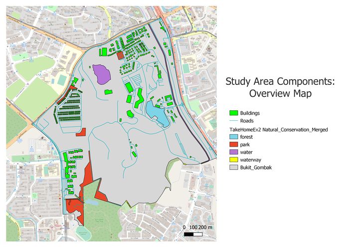
Part 1: Study Area Map Components
FIGURE I
Study Area Map Components
Firstly, the above summarises an overview of the study area and its map components we want to consider in this suitability land analysis for the Communicable Disease Quarantine Centre in Bukit Gombak.
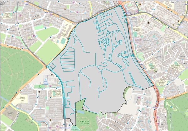
FIGURE II
Target Road Map
Figure II shows Bukit Gombak's Road Network that will be accounted in as an Accesibility factor in weighing the location suitability.
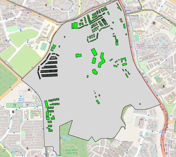
FIGURE III
Target Building Map
Figure III shows Bukit Gombak's Buildings that will be accounted in as an Health Risk factor in weighing the location suitability. We want the Disease Quarantine Centre to be further away from residential in order to ensure safe-zone. Health Risk factor will be prioritised as for the very fact that a Quarantine Centre exists, to ensure no further disease spreading. Bukit Gombak has mostly residential areas in its'subzone.
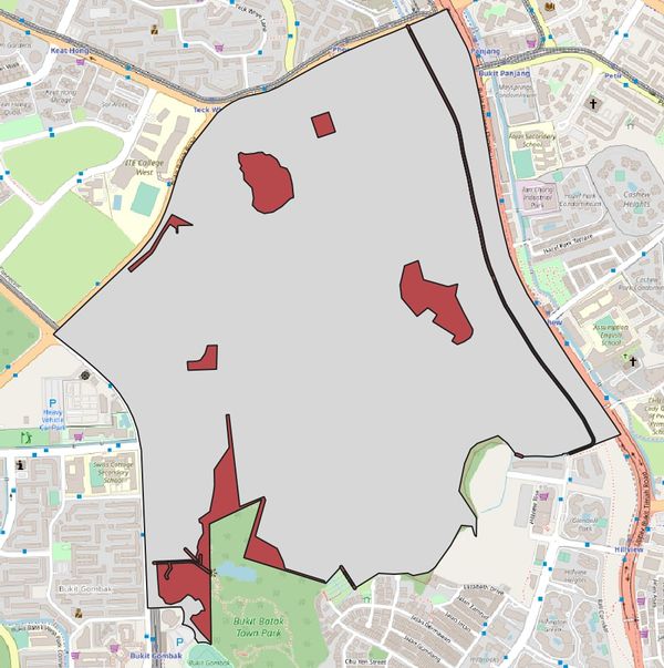
FIGURE III
Target Natural Features Map
FIGURE IV
Incomplete Waterway Target Inclusion. Applying buffering and merging of polygons in QGIS.
Figure IV shows Bukit Gombak's Natural Features that will be accounted in as an Natural Conservation factor in weighing the location suitability. The Natural features includes forest, park, water, and also waterway(canal, drain, stream). Waterway polygon was merged into the natural features in order to account in medium of disease transmission that could potentially cause disease spreading. We account this as risk factor that needed to be considered.
FIGURE V
Digital Elevation Map
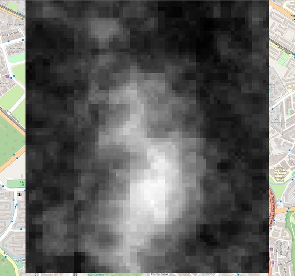
Figure V shows Bukit Gombak's Elevation Map that will be accounted in as an Economical factor in weighing the location suitability. Most projects will always assess its cost in building. In estimation, slope inclination of about 15 degrees and beyond could add further costs to increase significantly as the risks become greater and the work becomes more difficult to build.
Part 2: Study Area Proximity Maps
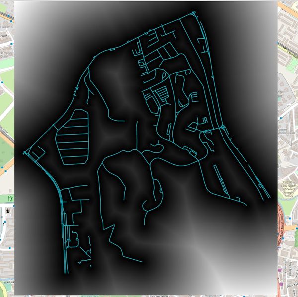
FIGURE VI
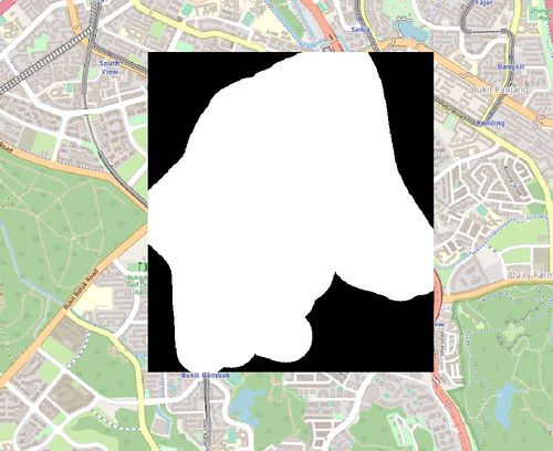
Accessibility Factor: Road Proximity Map
After target map elements have been rasterised. We perform the raster proximity distance on its layer and apply binary model classification on all the factor layers. The legend of Proximity map layer indicates that the furthest distance from the roads is 796.304 metres.
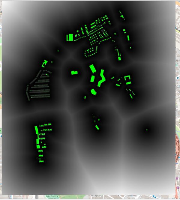
FIGURE VII
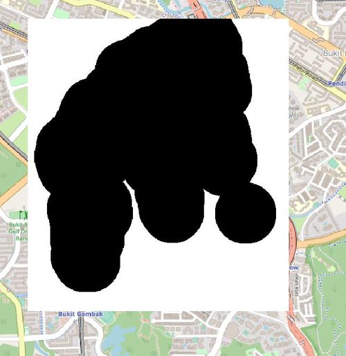
Health Risk Factor: Building Proximity Map
Applying the same methods used on road proximity map, The legend of Proximity map layer indicates that the furthest distance from the buildings is 910 metres.
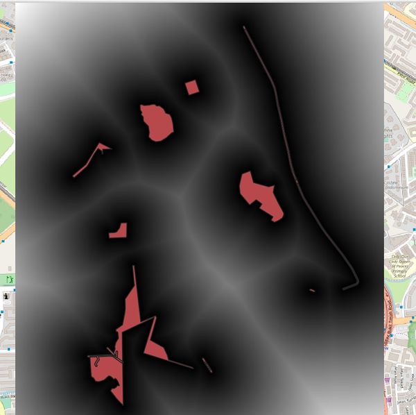
FIGURE VIII
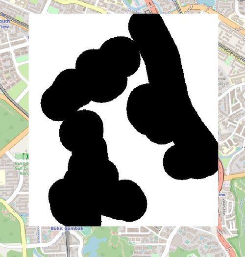
Natural Conservation Factor: Natural Features Proximity Map
Next, the Figure VIII shows the Natural Features Proximity Map where the legend of Proximity map layer indicates that the furthest distance from the natural features is 948.117 metres.
FIGURE IX
Economic Factor: Slope Layer
Lastly, Figure IX shows the slope layer. The legend of Slope layer shows that the minimum and maximum values of the slope values are 0 and 34.5339 degrees respectively.
Criterion Scores for Map Components
FIGURE X
Accesibility Factor: Road Binary & Criteria Score
Figure X includes the accesibility binary model, where we prefer location under 200 m.
FIGURE XI
Health Risk Factor: Building Binary & Criteria Score
The Figure XI includes the health risk binary model where we prefer that buildings are 250 meters away from the Disease Quarantine Centre.
FIGURE XII
Natural Conservation Factor: Natural Features Binary & Criteria Score
Next, Figure XII includes the natural conservation risk binary model, where we prefer public natural features and waterways are 200 meters away from the centre.
FIGURE XIII
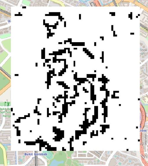
Economical Factor: Slope Binary & Criteria Score
Lastly, Figure XIII includes the economical factor binary model,where we locations where slope inclination is below or equal to 15 degrees.
Analytical Hierarchical Process Input Matrix & Approach
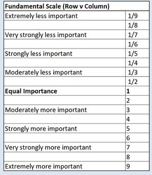
FIGURE XIV
SCB Associates' AHP Scoring Framework
The Analytical Hierachy Process provides a framework to assist the prioritisation of different factors in decision making. The method applies the pairwise comparison by evaluating relative importance of 2 factors. The matrix mathematics was applied in deriving appropriate weighting ratio by ensuring consistency ratio (consistency index/ratio index) is equal or less than 10%. Figure XIV shows the Pairwise comparson matrix's fundamental scale used.
FIGURE XV
AHP Scoring Framework for Accounting Factors
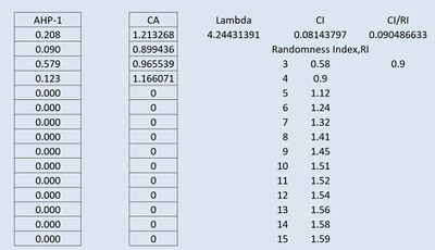
Next, we evaluate each factor with the corresponding grading scale in which the SCB's AHP model with automatically compute its consistency ratio. In summary, the priority that we will aim will be ensuring firstly that health risk is minimal. Second, the economic factor has to be reasonable as government facilities are built upon contribution of Singapore's citizen, thus we need to be accountable with every cent that we spent in developing the quarantine centre. Third, Natural Conservation comes next and Road Accessibility as the last priority. It would have been the best scenario to get the best of everything. However, when dealing in what we called as a VUCA world we live in, we have to be reasonable in determining whats a higher priority to be considered.
FIGURE XVI
AHP Results
The above reference listed on Figure XVI lists a summary of the AHP result. The desired consistency consistency rating was achieved thus we will proceed by applying this to the Binary model in identifying non-preferable location, good location, and best location based on this weighthing ratio.
FIGURE XVII
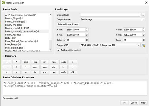
Weighing AHP Scores into QGIS Raster Calculator
Based on the derived factors ratio, we plot a binary raster model by computing ratio of the different factor binary models. Since each binary factor model uses a binary scale of 0 or 1. By applying the weighting scale, we will achieve a decimal metric of different preference where nearing number 1 will be the best case scenario.
FIGURE XVIII
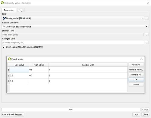
Reclassifying Raster Values using SAGA's Plugin for Degrees of Suitability
Lastly, we use the SAGA's Plugin to classify the degree of suitability unto 3 groups. Decimal 0 - 0.59 as not suitable location, 0.6 - 0.69 as good location, and 0.7 - 1 (inclusive) will the the best scenario.
Recommendation
FIGURE XIX
Suitability Map Overview
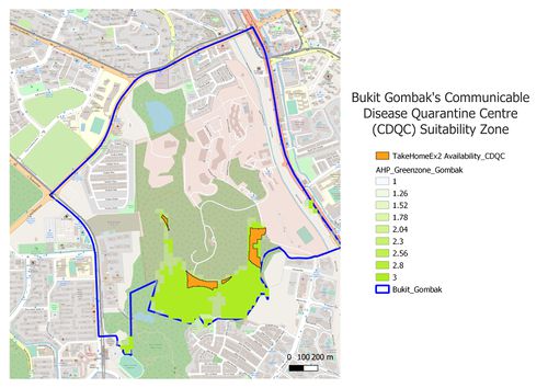
In this analysis for the quarantine centre land suitability. We used both the AHP weighting factor and also the simple standardised binary model at the raster calculator process in deriving locations. The simple standardised binary model was generated by performing an XOR method unto the different factor binary layer through multiplication. A case where a pixel (one area measurement of 5 x 5 m) has 0 value on its factor will be derived as a non preferable location. Next, the generated raster was transformed into a polygon through the Raster's Poligonize (Raster to Vector) function. 0 values pixels were eliminated thus only showing polygons that has 1 binary value or we take it as best location where it has meet all the given scenario as indicated by the orange polygon in Figure XIX.
On the other hand, the AHP weigthed binary model was visualised using a singleband pseudocolour where the best location (Metric value of 3) is indicated by the bright green zone and the good location (Metric location 2) was indicated by the lighter green pixel.
FIGURE XX
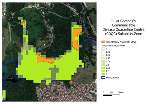
Qualitative Analysis: Zooming into Possible Region Using Google's Satelitte
Using qualitative obsevation method we can observe that most of the greenzone preferable location were located inside the Bukit Panjang Camp. This is a valid location as the location has a rather empty zones isolated from the factors we have mentioned earlier when determining the suitable location for quarantine disease. Figure XX, shows a zoomed overview of the green zone (best location) using the Google Satellite basemap. We can see that the proposed location is quite well fitted as its further away from public population. In addition, higher security level is achieved by building a quarantine zone in a protected and isolated location while still having road accessibility factor.
FIGURE XXI
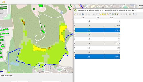
Making Recommendation based on Availibity of Land
However, there is still a bigger question to be ask in the possibility of this proposal. Will it be possible to integrate a quarantine centre within the Bukit Panjang Basecamp? Would this place our fellow soldiers in risk of being exposed if an unexpected breakout happens? Will political agenda will be a factor in this current quarantine centre proposal even when analysis has shown that its the most compatible location?
Another recommendation would be reallocating the bukit panjang camp's greenzone to another isolated zone just for the quarantine zone which will have a direct road network accessibility, thus quarantine zone will not techincally fall inside the bukit panjang camp zone as ensuring proper access will be difficult since both department has different needs of confidentiality and agendas.
