Difference between revisions of "SMT201 AY2019-20G2 Ex2 JerryTohvan"
| Line 1: | Line 1: | ||
| − | == Part 1: Study Area Map Components == | + | == Part 1: Study Area Map Components == |
[[File:Overview map.jpg|700px|center]] | [[File:Overview map.jpg|700px|center]] | ||
| Line 100: | Line 100: | ||
<br> | <br> | ||
<br> | <br> | ||
| − | After target map elements have been rasterised. We perform the raster proximity distance on its layer and apply binary model classification on all the factor layers. | + | After target map elements have been rasterised. We perform the raster proximity distance on its layer and apply binary model classification on all the factor layers. The legend of Proximity map layer indicates that the furthest distance from the roads is 796.304 metres. |
<br> | <br> | ||
<br> | <br> | ||
| Line 116: | Line 116: | ||
<br> | <br> | ||
<br> | <br> | ||
| − | Applying the same methods used on road proximity map, the | + | Applying the same methods used on road proximity map, The legend of Proximity map layer indicates that the furthest distance from the buildings is 910 metres. |
<br> | <br> | ||
<br> | <br> | ||
| Line 128: | Line 128: | ||
lang=EN-GB style='font-size:8.0pt;font-family:"Times New Roman",serif; | lang=EN-GB style='font-size:8.0pt;font-family:"Times New Roman",serif; | ||
mso-fareast-font-family:"Times New Roman";font-variant:small-caps;color:white'><span | mso-fareast-font-family:"Times New Roman";font-variant:small-caps;color:white'><span | ||
| − | style='color:windowtext'>Natural Conservation Factor | + | style='color:windowtext'>Natural Conservation Factor: Natural Features Proximity Map</span></span></p> |
<br> | <br> | ||
<br> | <br> | ||
<br> | <br> | ||
| − | Next, the Figure VIII | + | Next, the Figure VIII shows the Natural Features Proximity Map where the legend of Proximity map layer indicates that the furthest distance from the natural features is 948.117 metres. |
<br> | <br> | ||
<br> | <br> | ||
| Line 151: | Line 151: | ||
<br> | <br> | ||
<br> | <br> | ||
| − | Lastly, Figure IX | + | Lastly, Figure IX shows the slope layer. The legend of Slope layer shows that the minimum and maximum values of the slope values are 0 and 34.5339 degrees respectively. |
<br> | <br> | ||
<br> | <br> | ||
| Line 168: | Line 168: | ||
style='color:windowtext'>Accesibility Factor: Road Binary & Criteria Score</span></span></p> | style='color:windowtext'>Accesibility Factor: Road Binary & Criteria Score</span></span></p> | ||
<br> | <br> | ||
| + | <br> | ||
| + | Figure X includes the accesibility binary model, where we prefer location under 200 m. | ||
| + | <br><br> | ||
[[File:Binary buildings.jpg|500px|center]] | [[File:Binary buildings.jpg|500px|center]] | ||
| Line 180: | Line 183: | ||
style='color:windowtext'>Health Risk Factor: Building Binary & Criteria Score</span></span></p> | style='color:windowtext'>Health Risk Factor: Building Binary & Criteria Score</span></span></p> | ||
<br> | <br> | ||
| + | <br> | ||
| + | The Figure XI includes the health risk binary model where we prefer that buildings are 250 meters away from the Disease Quarantine Centre. | ||
| + | <br><br> | ||
[[File:Binary natural.jpg|500px|center]] | [[File:Binary natural.jpg|500px|center]] | ||
| Line 192: | Line 198: | ||
style='color:windowtext'>Natural Conservation Factor: Natural Features Binary & Criteria Score</span></span></p> | style='color:windowtext'>Natural Conservation Factor: Natural Features Binary & Criteria Score</span></span></p> | ||
<br> | <br> | ||
| − | + | <br> | |
| + | Next, Figure XII includes the natural conservation risk binary model, where we prefer public natural features and waterways are 200 meters away from the centre. | ||
| + | <br><br> | ||
[[File:Binary slope.jpg|500px|center]] | [[File:Binary slope.jpg|500px|center]] | ||
| Line 205: | Line 213: | ||
style='color:windowtext'>Economical Factor: Slope Binary & Criteria Score</span></span></p> | style='color:windowtext'>Economical Factor: Slope Binary & Criteria Score</span></span></p> | ||
<br> | <br> | ||
| − | + | <br> | |
| + | Lastly, Figure XIII includes the economical factor binary model,where we locations where slope inclination is below or equal to 15 degrees. | ||
| + | <br><br> | ||
== Analytical Hierarchical Process Input Matrix & Approach == | == Analytical Hierarchical Process Input Matrix & Approach == | ||
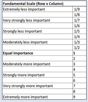
[[File:AHP Scale.jpg|300px|center]] | [[File:AHP Scale.jpg|300px|center]] | ||
Revision as of 00:51, 4 November 2019
Contents
Part 1: Study Area Map Components
FIGURE I
Study Area Map Components
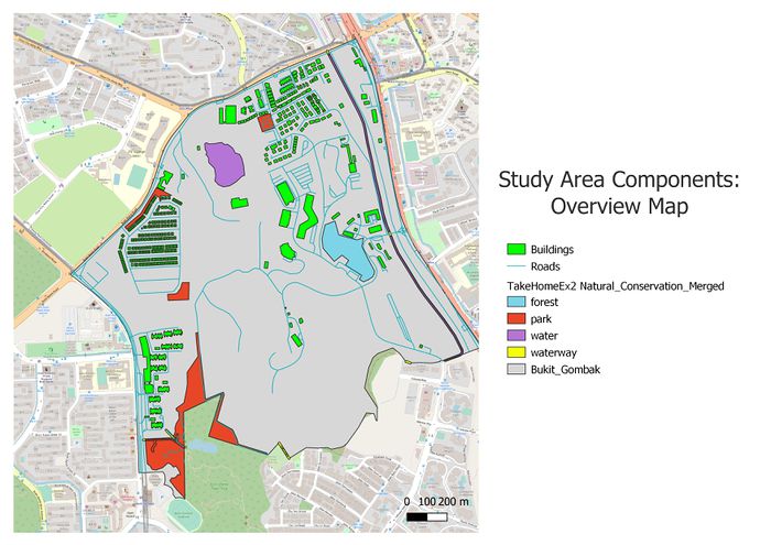
Firstly, the above summarises an overview of the study area and its map components we want to consider in this suitability land analysis for the Communicable Disease Quarantine Centre in Bukit Gombak.
FIGURE II
Target Road Map
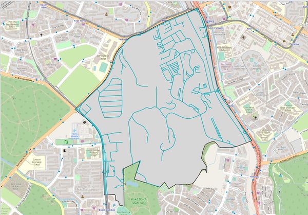
Figure II shows Bukit Gombak's Road Network that will be accounted in as an Accesibility factor in weighing the location suitability.
FIGURE III
Target Building Map
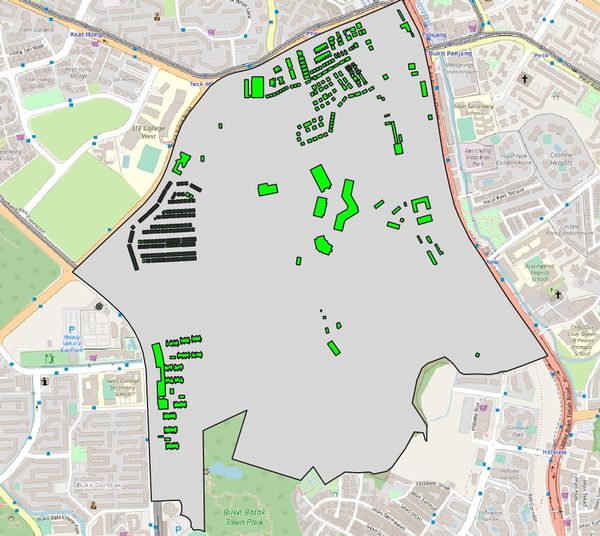
Figure III shows Bukit Gombak's Buildings that will be accounted in as an Health Risk factor in weighing the location suitability. We want the Disease Quarantine Centre to be further away from residential in order to ensure safe-zone. Health Risk factor will be prioritised as for the very fact that a Quarantine Centre exists, to ensure no further disease spreading. Bukit Gombak has mostly residential areas in its'subzone.
FIGURE III
Target Natural Features Map
FIGURE IV
Incomplete Waterway Target Inclusion. Applying buffering and merging of polygons in QGIS.
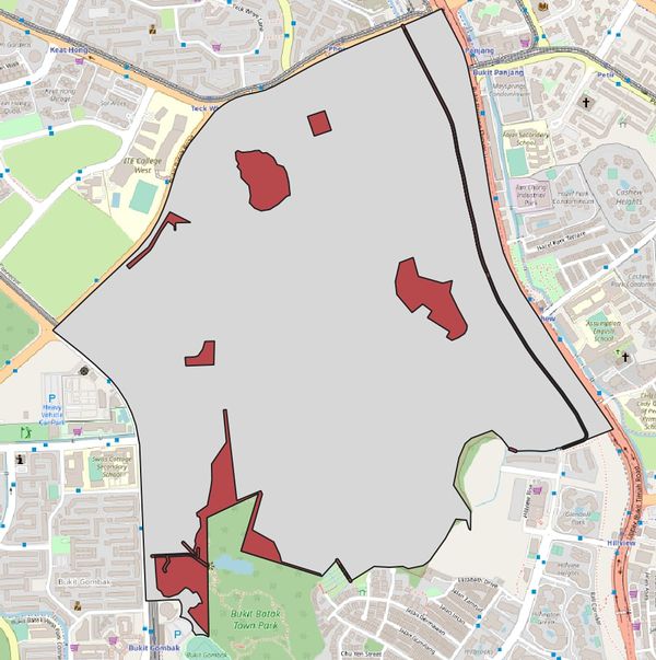
Figure IV shows Bukit Gombak's Natural Features that will be accounted in as an Natural Conservation factor in weighing the location suitability. The Natural features includes forest, park, water, and also waterway(canal, drain, stream). Waterway polygon was merged into the natural features in order to account in medium of disease transmission that could potentially cause disease spreading. We account this as risk factor that needed to be considered.
FIGURE V
Digital Elevation Map
Figure V shows Bukit Gombak's Elevation Map that will be accounted in as an Economical factor in weighing the location suitability. Most projects will always assess its cost in building. In estimation, slope inclination of about 15 degrees and beyond could add further costs to increase significantly as the risks become greater and the work becomes more difficult to build.
Part 2: Study Area Proximity Maps
FIGURE VI
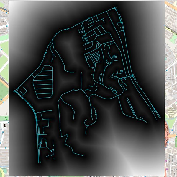
Accessibility Factor: Road Proximity Map
After target map elements have been rasterised. We perform the raster proximity distance on its layer and apply binary model classification on all the factor layers. The legend of Proximity map layer indicates that the furthest distance from the roads is 796.304 metres.
FIGURE VII
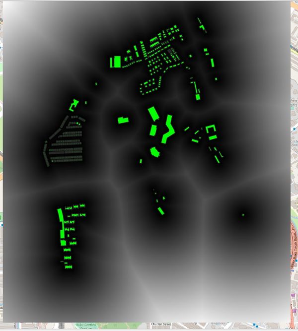
Health Risk Factor: Building Proximity Map
Applying the same methods used on road proximity map, The legend of Proximity map layer indicates that the furthest distance from the buildings is 910 metres.
FIGURE VIII
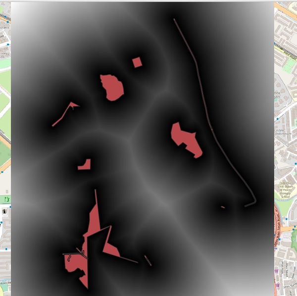
Natural Conservation Factor: Natural Features Proximity Map
Next, the Figure VIII shows the Natural Features Proximity Map where the legend of Proximity map layer indicates that the furthest distance from the natural features is 948.117 metres.
FIGURE IX
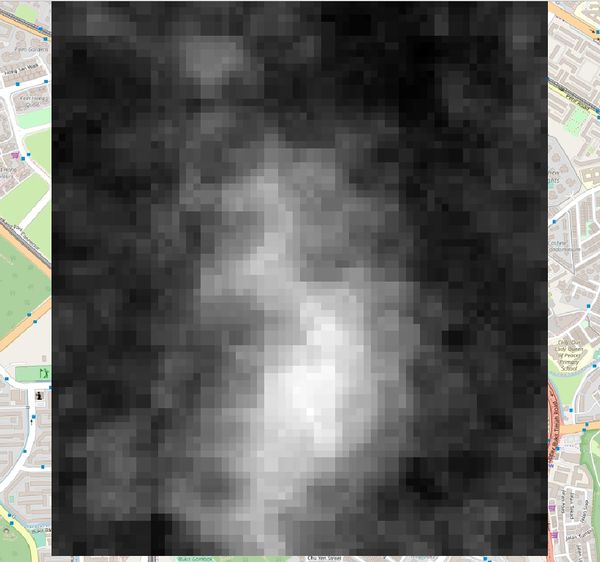
Economic Factor: Slope Layer
Lastly, Figure IX shows the slope layer. The legend of Slope layer shows that the minimum and maximum values of the slope values are 0 and 34.5339 degrees respectively.
Criterion Scores for Map Components
FIGURE X
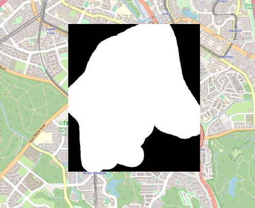
Accesibility Factor: Road Binary & Criteria Score
Figure X includes the accesibility binary model, where we prefer location under 200 m.
FIGURE XI
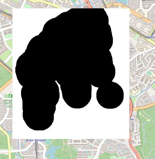
Health Risk Factor: Building Binary & Criteria Score
The Figure XI includes the health risk binary model where we prefer that buildings are 250 meters away from the Disease Quarantine Centre.
FIGURE XII
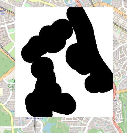
Natural Conservation Factor: Natural Features Binary & Criteria Score
Next, Figure XII includes the natural conservation risk binary model, where we prefer public natural features and waterways are 200 meters away from the centre.
FIGURE XIII
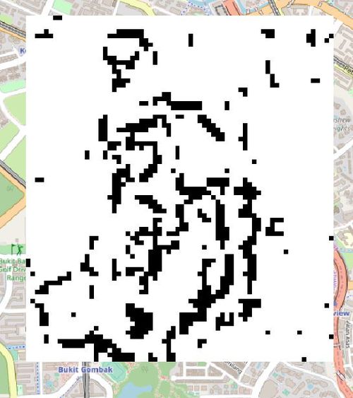
Economical Factor: Slope Binary & Criteria Score
Lastly, Figure XIII includes the economical factor binary model,where we locations where slope inclination is below or equal to 15 degrees.
Analytical Hierarchical Process Input Matrix & Approach
FIGURE XIV
SCB Associates' AHP Scoring Framework
FIGURE XV
AHP Scoring Framework for Accounting Factors
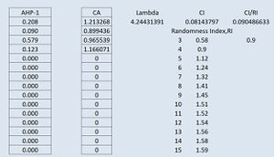
FIGURE XVI
AHP Results
FIGURE XVII
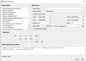
Weighing AHP Scores into QGIS Raster Calculator
FIGURE XVIII
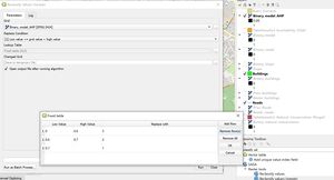
Reclassifying Raster Values using SAGA's Plugin for Degrees of Suitability
Recommendation
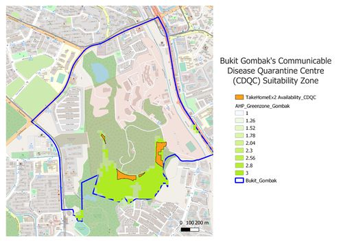
FIGURE XIX
Suitability Map Overview
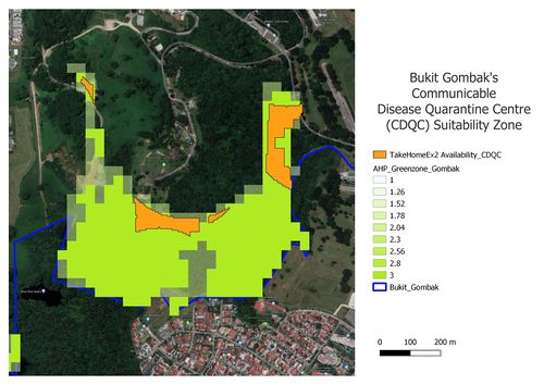
FIGURE XX
Qualitative Analysis: Zooming into Possible Region Using Google's Satelitte
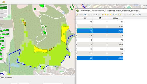
FIGURE XXI
Making Recommendation based on Availibity of Land
