Difference between revisions of "SMT201 AY2019-20G2 Ex1 Soh Bai He"
| (6 intermediate revisions by the same user not shown) | |||
| Line 9: | Line 9: | ||
'''Handling of Data:''' general-information-of-schools.csv is geocoded into school_information.shp using geocode.py | '''Handling of Data:''' general-information-of-schools.csv is geocoded into school_information.shp using geocode.py | ||
<br><br> | <br><br> | ||
| − | Choice of Classification:'''<br> | + | '''Choice of Classification:'''<br> |
1) Categorisation by school type (school_type). Junior College and Centralised Institute are grouped together as both offers pre-university courses and lead to the ‘A’ Level examinations.<br> | 1) Categorisation by school type (school_type). Junior College and Centralised Institute are grouped together as both offers pre-university courses and lead to the ‘A’ Level examinations.<br> | ||
2) Categorisation by region to facilitate easier visualisation of the distribution of schools by region. | 2) Categorisation by region to facilitate easier visualisation of the distribution of schools by region. | ||
<br><br> | <br><br> | ||
| − | '''Visual Variable:''' | + | '''Visual Variable:''' SVG marker of a book is used to symbolise schools. Different colours are used for each school type/region for easier identification. |
<br><br> | <br><br> | ||
'''Feature count:''' Total (344), Primary (181), Secondary (138), Mixed Level (14), Junior College/Centralised Institute (11) | '''Feature count:''' Total (344), Primary (181), Secondary (138), Mixed Level (14), Junior College/Centralised Institute (11) | ||
| Line 49: | Line 49: | ||
[[File:Land use.jpg|800px|thumb|center|Data Source: data.gov.sg / File: G_MP14_LAND_USE_PL.shp]] | [[File:Land use.jpg|800px|thumb|center|Data Source: data.gov.sg / File: G_MP14_LAND_USE_PL.shp]] | ||
<br> | <br> | ||
| − | '''Choice of Classification:''' Categorisation by type of land use (LU_DESC). To minimise the number of categories and colours that might overwhelm the user, several sub categories of the same type of development are grouped into | + | '''Choice of Classification:''' Categorisation by type of land use (LU_DESC). To minimise the number of categories and colours that might overwhelm the user, several sub categories of the same type of development are grouped into its main category. <br><br> |
'''Visual Variable:''' Colour fill as the respective type of land use. I referenced [https://www.ura.gov.sg/Corporate/Planning/Concept-Plan/Past-Concept-Plans URA’s Past Concept Plan] colours for each development. Planning areas are labelled to aid in the visualisation of the distribution of land use in Singapore.<br><br> | '''Visual Variable:''' Colour fill as the respective type of land use. I referenced [https://www.ura.gov.sg/Corporate/Planning/Concept-Plan/Past-Concept-Plans URA’s Past Concept Plan] colours for each development. Planning areas are labelled to aid in the visualisation of the distribution of land use in Singapore.<br><br> | ||
'''Observation:''' The West region is dominated by industrial developments along with the Western Water Catchment. There are fewer residential areas in the West, however, a new HDB town called Tengah will be built soon. | '''Observation:''' The West region is dominated by industrial developments along with the Western Water Catchment. There are fewer residential areas in the West, however, a new HDB town called Tengah will be built soon. | ||
| Line 60: | Line 60: | ||
<br> | <br> | ||
'''2010 Data: SUBZONE_AGE_GENDER_2010.shp'''<br> | '''2010 Data: SUBZONE_AGE_GENDER_2010.shp'''<br> | ||
| − | <pre>(A): Computed column ‘Above65’ which sums up the number of aged per subzone | + | <pre>(for Part A): Computed column ‘Above65’ which sums up the number of aged per subzone |
| − | (B): Computed column ‘Aged_Pptn’ using the formula (Above65/TOTAL)*100</pre | + | (for Part B): Computed column ‘Aged_Pptn’ using the formula (Above65/TOTAL)*100</pre><br> |
'''2018 Data: SGResidentPopulationAgeGroupSex_2018.csv'''<br> | '''2018 Data: SGResidentPopulationAgeGroupSex_2018.csv'''<br> | ||
| − | Data cleaning is performed on excel and saved as SGResidentPopulationAgeGroupSex_2018_cleaned.csv. ‘ZONE_N’ and ‘SUBZONE_N’ are converted to uppercase to match the data in MP14_Subzone. Null values are replaced with 0. After data | + | Data cleaning is performed on excel and saved as SGResidentPopulationAgeGroupSex_2018_cleaned.csv. ‘ZONE_N’ and ‘SUBZONE_N’ are converted to uppercase to match the data in MP14_Subzone. Null values are replaced with 0. After the data is cleaned, it is joined with MP14_Subzone by ‘SUBZONE_N’. <br> |
<pre> | <pre> | ||
| − | (A): Computed column ‘SG2018_AGED_TOTAL’ which sums up the number of aged per subzone. | + | (for Part A): Computed column ‘SG2018_AGED_TOTAL’ which sums up the number of aged per subzone. |
| − | (B): Computed column ‘SG2018_AGED_PPTN’ using the formula (SG2018_AGED_TOTAL/SG2018_TOTAL)*100 | + | (for Part B): Computed column ‘SG2018_AGED_PPTN’ using the formula (SG2018_AGED_TOTAL/SG2018_TOTAL)*100 |
| − | (C): Both the 2010 and 2018 data are joined together by ‘SUBZONE_N’. Computed column ‘Change’ using the formula (SG2018_AGED_TOTAL - Above65)/Above65 </pre | + | (for Part C): Both the 2010 and 2018 data are joined together by ‘SUBZONE_N’. Computed column ‘Change’ using the formula (SG2018_AGED_TOTAL - Above65)/Above65 </pre><br> |
| − | When there is | + | When there is null values during the computation of the new columns, I replaced them with 0. The computed column is then used as the classification variable for each part. I chose to classify by Graduated symbol with Natural Breaks (Jenks) as the classes are based on natural groupings inherent in the data. For a clearer visualisation, I used single colour ramps for each map. |
| − | === A: Aged | + | === A: Count of Aged Population (+65) in 2010 and 2018 === |
<br> | <br> | ||
[[File:P2a-2010.jpg|800px|thumb|center|Data Source: data.gov.sg / File: SUBZONE_AGE_GENDER_2010.shp]] | [[File:P2a-2010.jpg|800px|thumb|center|Data Source: data.gov.sg / File: SUBZONE_AGE_GENDER_2010.shp]] | ||
| Line 80: | Line 80: | ||
| − | === B: | + | === B: Proportion of Aged Population in 2010 and 2018 === |
<br> | <br> | ||
[[File:P2b-2010.jpg|800px|thumb|center|Data Source: data.gov.sg / File: SUBZONE_AGE_GENDER_2010.shp]] | [[File:P2b-2010.jpg|800px|thumb|center|Data Source: data.gov.sg / File: SUBZONE_AGE_GENDER_2010.shp]] | ||
| Line 89: | Line 89: | ||
| − | === C: Percentage change of | + | === C: Percentage change of Aged Population between 2010 and 2018 === |
<br> | <br> | ||
[[File:P2c.jpg|800px|thumb|center|Data Source: data.gov.sg, singstat.gov.sg / File: SUBZONE_AGE_GENDER_2010.shp, SGResidentPopulationAgeGroupSex_2018.csv ]] | [[File:P2c.jpg|800px|thumb|center|Data Source: data.gov.sg, singstat.gov.sg / File: SUBZONE_AGE_GENDER_2010.shp, SGResidentPopulationAgeGroupSex_2018.csv ]] | ||
Latest revision as of 22:55, 15 September 2019
Part One: Thematic Mapping
Public Education Institutions
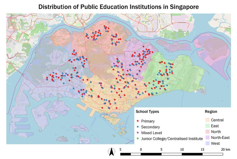
Handling of Data: general-information-of-schools.csv is geocoded into school_information.shp using geocode.py
Choice of Classification:
1) Categorisation by school type (school_type). Junior College and Centralised Institute are grouped together as both offers pre-university courses and lead to the ‘A’ Level examinations.
2) Categorisation by region to facilitate easier visualisation of the distribution of schools by region.
Visual Variable: SVG marker of a book is used to symbolise schools. Different colours are used for each school type/region for easier identification.
Feature count: Total (344), Primary (181), Secondary (138), Mixed Level (14), Junior College/Centralised Institute (11)
Observation: Of all school types, Junior College/Centralised Institute has the least number. However, the existing ones are well distributed across Singapore with every region covered.
Road Network System
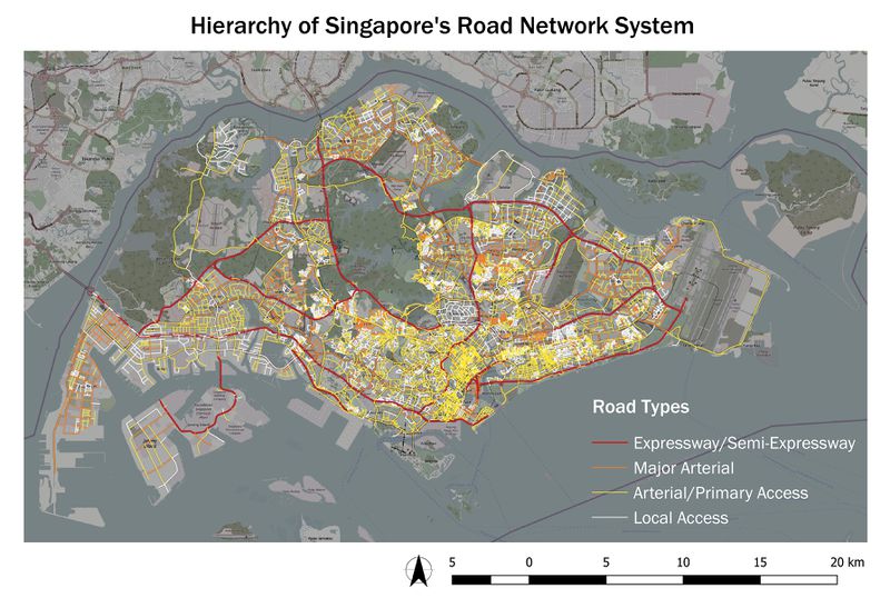
Handling of Data & Choice of Classification: RoadSectionLine.shp is exported into .csv format and new columns RD_CAT_NO, RD_MAIN_CAT are added on excel (road-section-category-sorted.csv). Roads are then sorted with reference to the table below. Thereafter, I analysed the remaining roads (that do not include the street name descriptors in the table below) on the OpenStreetMap and grouped them into Arterial/Primary Access as they are minor roads that provide access to developments.
| Road Category | Street Name Descriptor |
|---|---|
| Expressway and Semi-Expressway (Cat 1) | Expressway, Highway, Parkway |
| Major Arterial (Cat 2) | Boulevard, Avenue, Way |
| Arterial & Primary Access (Cat 3 & 4) | Drive, Street, Road |
| Local Access Roads (Cat 5) | Walk, Lane, Link |
Visual Variable: Line symbols with different colours are used to represent each road type. A warm colour scheme (red > orange > yellow > white) is chosen to highlight the hierarchy of road types. Expressway is given the thickest width as they form the primary network in the road system.
2014 Master Plan Landuse
Choice of Classification: Categorisation by type of land use (LU_DESC). To minimise the number of categories and colours that might overwhelm the user, several sub categories of the same type of development are grouped into its main category.
Visual Variable: Colour fill as the respective type of land use. I referenced URA’s Past Concept Plan colours for each development. Planning areas are labelled to aid in the visualisation of the distribution of land use in Singapore.
Observation: The West region is dominated by industrial developments along with the Western Water Catchment. There are fewer residential areas in the West, however, a new HDB town called Tengah will be built soon.
Part Two: Choropleth Mapping
Discussion (Handling of Data, Classification Choices)
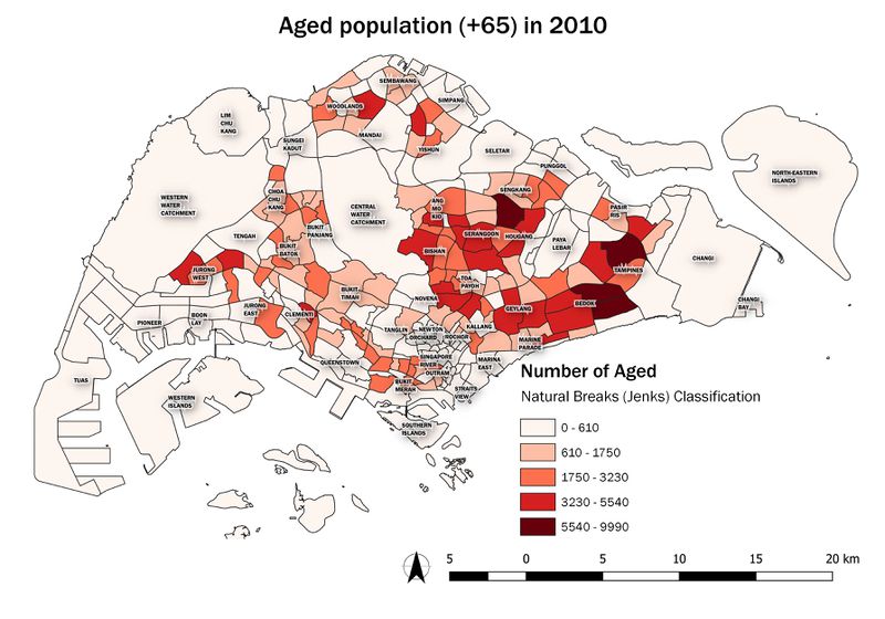
2010 Data: SUBZONE_AGE_GENDER_2010.shp
(for Part A): Computed column ‘Above65’ which sums up the number of aged per subzone
(for Part B): Computed column ‘Aged_Pptn’ using the formula (Above65/TOTAL)*100
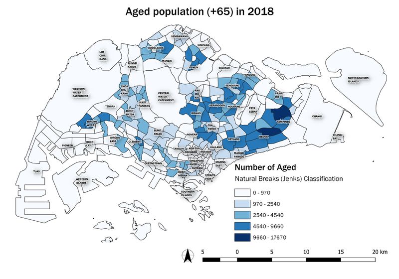
2018 Data: SGResidentPopulationAgeGroupSex_2018.csv
Data cleaning is performed on excel and saved as SGResidentPopulationAgeGroupSex_2018_cleaned.csv. ‘ZONE_N’ and ‘SUBZONE_N’ are converted to uppercase to match the data in MP14_Subzone. Null values are replaced with 0. After the data is cleaned, it is joined with MP14_Subzone by ‘SUBZONE_N’.
(for Part A): Computed column ‘SG2018_AGED_TOTAL’ which sums up the number of aged per subzone.
(for Part B): Computed column ‘SG2018_AGED_PPTN’ using the formula (SG2018_AGED_TOTAL/SG2018_TOTAL)*100
(for Part C): Both the 2010 and 2018 data are joined together by ‘SUBZONE_N’. Computed column ‘Change’ using the formula (SG2018_AGED_TOTAL - Above65)/Above65
When there is null values during the computation of the new columns, I replaced them with 0. The computed column is then used as the classification variable for each part. I chose to classify by Graduated symbol with Natural Breaks (Jenks) as the classes are based on natural groupings inherent in the data. For a clearer visualisation, I used single colour ramps for each map.
A: Count of Aged Population (+65) in 2010 and 2018
There is a growing trend in the number of aged, such that the range has increased to over 10000 from 2010 to 2018. The East and North-East regions have a high aged population density, where sub-regions Bedok North (15160) and Tampines East (17670) house the highest number of aged in 2018.
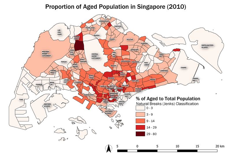
B: Proportion of Aged Population in 2010 and 2018
In contrast to the count of aged population in (A), the proportion of aged population shows that the Central region has a higher aged population density. Proportion of aged population is a more accurate representation of population density as it considers the total population per sub-region.
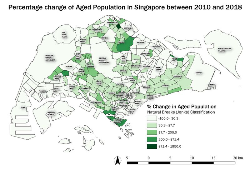
C: Percentage change of Aged Population between 2010 and 2018
Although there are subzones with negative change in aged population, more than half of the subzones faced a positive increase in aged population. It is surprising that the Southern Islands have a high increase in aged population.
References
Urban Redevelopment Authority’s Handbook on Guidelines for Naming of Streets
Urban Redevelopment Authority’s Past Concept Plan
