Difference between revisions of "Group06 Elec3city Proposal"
Yu.fu.2015 (talk | contribs) |
Yu.fu.2015 (talk | contribs) |
||
| (82 intermediate revisions by 3 users not shown) | |||
| Line 4: | Line 4: | ||
{| style="background-color:#ffffff ; margin: 3px 10px 3px 10px; width="80%"| | {| style="background-color:#ffffff ; margin: 3px 10px 3px 10px; width="80%"| | ||
| − | | style="font-family:Open Sans, Arial, sans-serif; font-size:15px; text-align: center; border-top:solid #ffffff; border-bottom:solid #f5f5f5" width=" | + | | style="font-family:Open Sans, Arial, sans-serif; font-size:15px; text-align: center; border-top:solid #ffffff; border-bottom:solid #f5f5f5" width="210px" | |
[[Elec3city|<font color="#3c3c3c"><strong>HOME</strong></font>]] | [[Elec3city|<font color="#3c3c3c"><strong>HOME</strong></font>]] | ||
| Line 28: | Line 28: | ||
<div style="text-align: left; direction: ltr; margin-left: 1em;"> | <div style="text-align: left; direction: ltr; margin-left: 1em;"> | ||
| − | + | Rising energy consumption is an issue that plagues the Singapore government for several years. Recently, the government has begun pushing for more efficient energy usage, and most effort is expended on the efficiency of energy sources – e.g. using less carbon-intensive fuels. In exploring potential ways to aid this cause, we realised that there has been scant statistical analysis energy consumption patterns. As such, our team feels that there is a need for an app which allows for authorities in Singapore such as the National Environment Agency to understand with data-driven evidence the origins of variation in Singapore energy consumption, so as to allow for more targeted efforts to reduce energy wastage. Another factor that provided a fertile ground for the development of this application is the availability of energy consumption data, with granularity right down to individual postal code. | |
| + | |||
</div> | </div> | ||
| − | + | ||
== Project Objective == | == Project Objective == | ||
| − | <div style="text-align: left; direction: ltr; margin-left: 1em;"> | + | <div style="text-align: left; direction: ltr; margin-left: 1em;"> |
| − | + | We have been observing rising trends in energy consumption across all sub-sectors, including households, which has seen sharp increase over the years from 6092.5GWh in 2005 to 7295.8GWh in 2017. As such, household sub-sector is a good starting point for our analysis. | |
| − | + | ||
| − | + | *Energy Consumption Patterns in Singapore | |
| − | + | Through the exploration of potential energy consumption patterns among households in Singapore, we will be able to tease out potential drivers of energy consumption. We will not only be looking at seasonal patterns in consumption (i.e. Is there a particular month in a year when energy consumption spikes?), we will also try to identify spatial patterns in consumption (i.e. Is there a particular region in Singapore whereby energy consumption is particularly high?). | |
| + | |||
| + | *Temperature VS Energy Consumption | ||
| + | The next issue that we are interested in exploring is the relationship between temperature and energy consumption. Intuitively, we will assume that as temperature increases, energy consumption will also increase due to more electrical appliances used to regulate temperature such as air-conditioner. Thus, we plan to explore the relationship between temperature in different region of Singapore, and how this will affect the energy consumption in each respective region. | ||
| + | |||
| + | |||
</div> | </div> | ||
<br/> | <br/> | ||
| − | == Data | + | |
| + | == Data == | ||
{| class="wikitable" | {| class="wikitable" | ||
|- | |- | ||
! Data !! Source !! Data Type | ! Data !! Source !! Data Type | ||
|- | |- | ||
| − | |[https://www.ema.gov.sg/cmsmedia/Publications_and_Statistics/Statistics/52RSU.xls Average Monthly Household Electricity Consumption by Postal Code (Public Housing) & Dwelling Type, 2H 2016] ||ema.gov.sg || xls | + | |[https://www.ema.gov.sg/cmsmedia/Publications_and_Statistics/Statistics/52RSU.xls Average Monthly Household Electricity Consumption by Postal Code (Public Housing) & Dwelling Type, 2H 2016] ||Energy Market Authority (ema.gov.sg)|| xls |
|- | |- | ||
| − | | || | + | |[https://www.ema.gov.sg/cmsmedia/Publications_and_Statistics/Statistics/51RSU.xls Average Monthly Household Electricity Consumption by Postal Code (Public Housing) & Dwelling Type, 1H 2016] ||Energy Market Authority (ema.gov.sg)|| xls |
|- | |- | ||
| − | | || | + | |[https://www.ema.gov.sg/cmsmedia/Publications_and_Statistics/Statistics/25RSU.xls Average Monthly Household Electricity Consumption by Postal Code (Public Housing) & Dwelling Type, 2H 2015] ||Energy Market Authority (ema.gov.sg)|| xls |
|- | |- | ||
| − | | || | + | |[https://www.ema.gov.sg/cmsmedia/Publications_and_Statistics/Statistics/23RSU.xls Average Monthly Household Electricity Consumption by Postal Code (Public Housing) & Dwelling Type, 1H 2015] ||Energy Market Authority (ema.gov.sg)|| xls |
|- | |- | ||
| − | | || | + | |[https://www.ema.gov.sg/cmsmedia/Publications_and_Statistics/Statistics/MSA21.xls Average Monthly Household Electricity Consumption by Postal Code (Public Housing) & Dwelling Type, 2H 2014] ||Energy Market Authority (ema.gov.sg)|| xls |
|- | |- | ||
| − | | || | + | |[https://www.ema.gov.sg/cmsmedia/Publications_and_Statistics/Statistics/MSA17.xls Average Monthly Household Electricity Consumption by Postal Code (Public Housing) & Dwelling Type, 1H 2014] ||Energy Market Authority (ema.gov.sg)|| xls |
|- | |- | ||
| − | | || | + | |[https://www.ema.gov.sg/cmsmedia/Publications_and_Statistics/Statistics/MSA18.xls Average Monthly Household Electricity Consumption by Postal Code (Public Housing) & Dwelling Type, 2H 2013 ] ||Energy Market Authority (ema.gov.sg)|| xls |
|- | |- | ||
| − | | || | + | |[https://www.ema.gov.sg/cmsmedia/Publications_and_Statistics/Statistics/MSA16.xls Average Monthly Household Electricity Consumption by Postal Code (Public Housing) & Dwelling Type, 1H 2013] ||Energy Market Authority (ema.gov.sg)|| xls |
|- | |- | ||
| − | | || | + | |[https://www.ema.gov.sg/cmsmedia/Publications_and_Statistics/Statistics/2RSU.xls Average Monthly Household Electricity Consumption by Postal Code (Private Apartments), 2015 and 2016] ||Energy Market Authority (ema.gov.sg)|| xls |
|- | |- | ||
| − | | | + | |[https://www.ema.gov.sg/cmsmedia/Publications_and_Statistics/Statistics/22RSU.xls Average Monthly Household Electricity Consumption by Postal Code (Private Apartments), 2013 to 2014] ||Energy Market Authority (ema.gov.sg)|| xls |
| − | |||
| − | |||
| − | |||
| − | |||
| − | |||
| − | |||
| − | |||
| − | |||
| − | |||
| − | |||
| − | |||
| − | |||
| − | |||
| − | |||
| − | |||
| − | |||
| − | | | ||
| − | |||
| − | | | ||
| − | | | ||
| − | |||
| − | |||
|- | |- | ||
| − | | | + | |[https://www.singstat.gov.sg/-/media/files/publications/ghs/ghs2015/excel/t148-152.xls Resident Households by Planning Area and Dwelling Type/Household Size/Monthly Household Income] ||Department of Statistics Singapore (singstat.gov.sg)|| xls |
|- | |- | ||
| − | | | + | |[https://www.singstat.gov.sg/-/media/files/find_data/population/statistical_tables/respopagsex2000to2018.zip Singapore Residents by Planning Area/Subzone, Age Group and Sex, June 2000 - 2018] ||Department of Statistics Singapore (singstat.gov.sg)|| csv |
|- | |- | ||
| − | | | + | |[https://www.singstat.gov.sg/-/media/files/find_data/population/statistical_tables/respoptod2000to2018.zip Singapore Residents by Planning Area/Subzone and Type of Dwelling, June 2000 - 2018] ||Department of Statistics Singapore (singstat.gov.sg)|| csv |
|- | |- | ||
| − | | | + | |[http://www.weather.gov.sg/climate-historical-daily Singapore Climate Historical Data - crawled to get temperature and rain data from 2013 to 2016 at daily granularity] ||Meteorological Service Singapore (weather.gov.sg)|| csv |
|} | |} | ||
| − | + | == Literature Review == | |
| + | <div style="text-align: left; direction: ltr; margin-left: 1em;"> | ||
| + | In our due diligence for the project, the team looked at multiple research papers to inform and influence us in the best practices for analyzing geospatial variation in energy use, when it is to be compared against variables such as temperature and housing composition. | ||
| − | <br/> | + | <strong>1. Appropriate use of Interpolation Methods in GIS - Mitas, L. and Mitasova, H. Spatial Interpolation, Chap. 34 Spatial Interpolation (2005) </strong><br/><hr/> |
| − | |||
| − | < | ||
| − | |||
| − | |||
| − | + | <strong>Aim of literature:</strong> to enlighten reader of the appropriate interpolation method for different GIS themes. | |
| − | + | <br/><br/> | |
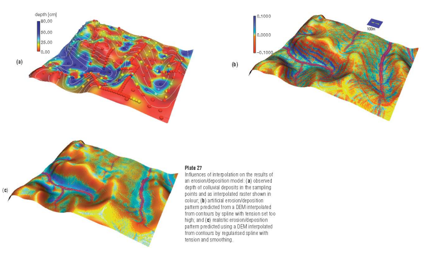
| − | + | [[File:Spline new edit.png|200px|framed|center|Comparison of Digital Elevation Models computed from contours, splines with tension and stream enforcement, and by regularised spline with tension (RST)]] | |
| − | |||
| − | |||
| − | [[File: | ||
| − | |||
| − | |||
<br/> | <br/> | ||
| − | |||
| − | + | <strong>Methodology:</strong><br/> | |
| − | + | 1. Inverse Distance Weighted Interpolation (IDW) - <u><b>adopted</b></u><br/> | |
| − | + | 2. Kriging - <i><b>rejected</b></i><br/> | |
| − | + | 3. Regularised spline with tension (RST) - <i><b>rejected</b></i><br/> | |
| − | |||
| − | |||
| − | |||
| − | |||
| − | |||
| − | |||
| − | |||
| − | <br/> | ||
| − | |||
| − | |||
| − | |||
| − | |||
| − | |||
| − | |||
| − | |||
| − | < | ||
| − | |||
| − | |||
| − | < | ||
| − | |||
<br/><br/> | <br/><br/> | ||
| − | <strong> | + | <strong>Learning Points:</strong><br/> |
| − | + | 1. Inverse Distance Weighted Interpolation (IDW) | |
| − | + | * Pro: relatively less demanding computationally | |
| − | + | * Pro: better at reproducing approximations on linear patterns | |
| − | + | * Con: "produces local extrema at the data points" | |
<br/> | <br/> | ||
| − | + | 2. Kriging | |
| − | < | + | * Con: While good at predicting spatial distribution of uncertainty, it is less successful for applications where <b>local geometry</b> and <b>smoothness</b> are the key issues - Critical weakness for our interpolation of temperature data where granularity is at housing block level, thus Kriging is rejected. |
| − | |||
| − | |||
| − | |||
| − | |||
| − | |||
| − | |||
<br/> | <br/> | ||
| − | + | 3. Regularised spline with tension (RST) | |
| − | + | * Pro: Allows for smoothing according to parameters such as the tension φ and smoothing weights {wj} which are empirically informed through minimisation of the predictive error estimated by a cross-validation procedure | |
| − | * | + | * Pro: Can realistically represent rough gradients in spite of the smoothness condition, if the roughness is sufficiently described by the input data - might be true of temperature when it comes to the Urban Heat Island effect - pockets of high building density can cause a micro-climate of higher temperatures; particularly pertinent in Singapore. |
| − | * | + | * Con: requires a lot of 'guess-timation' and past domain knowledge to fine-tune the tension and smoothing weights. |
<br/> | <br/> | ||
<strong>Areas for improvement:</strong><br/> | <strong>Areas for improvement:</strong><br/> | ||
| − | + | Our team has selected <b>IDW</b> as the interpolation technique for smoothing of temperature data of the 22 weather stations across Singapore. | |
| − | |||
<br/><br/> | <br/><br/> | ||
| + | <strong>2. A Spatial Analysis of the Relationship between Vegetation and Poverty - Dawson T., Sandoval J.S., Sagan V. and Crawford T. (2018)</strong><br/><hr/> | ||
| − | + | <strong>Aim of literature:</strong> investigate poverty and inequities that are associated with vegetation | |
| − | <strong>Aim of | ||
| − | [[File: | + | <br/><br/> |
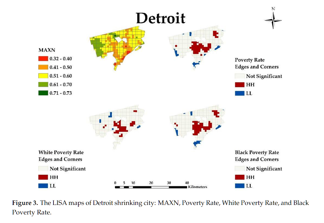
| + | [[File:Detroit lisa.png|200px|framed|center|Geospatial Visualisation of MAXN (regression coefficient for the time variable showing trend in Normalized Difference Vegetation Index) against race poverty geospatial distribution]] | ||
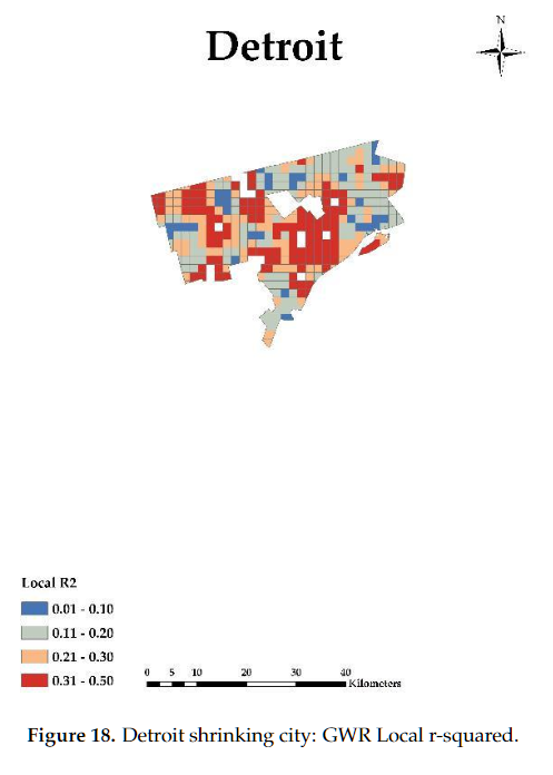
| + | [[File:Detroit gwr localrsquared.png|200px|framed|center|Local R-Squared values of model in Detroit]] | ||
<br/> | <br/> | ||
| − | |||
<strong>Methodology:</strong><br/> | <strong>Methodology:</strong><br/> | ||
| − | 1. | + | 1. Pixel level regression - Curve Fit extension in ArcGIS |
| − | * | + | * Run regression trend analysis using raster datasets for temporal analysis |
| − | 2. | + | 2. Global Ordinary Least Squares (OLS) regression |
| − | * | + | * Capture global geospatial correlation |
| − | 3. | + | 3. Local Geographically Weighted Regression (GWR) |
| − | + | * Capture local geospatial correlation | |
| − | * | + | 4. Moran's I for spatial autocorrelation |
| + | * For local level analysis of spatial autocorrelation | ||
| + | 5. Local Indicators of Spatial Association (LISA) map - Contiguity Edges and Corners method | ||
| + | * Queen contiguity to show clustering | ||
<br/> | <br/> | ||
| − | |||
<strong>Learning Points:</strong><br/> | <strong>Learning Points:</strong><br/> | ||
| − | + | 1. Pixel level regression - Curve Fit extension in ArcGIS | |
| − | + | * Helps us see the degree of model prediction for energy consumption given our variables | |
| − | * | + | 2. Global Ordinary Least Squares (OLS) regression |
| − | * We | + | * Investigate if the distributions of these random variables all have the same variance and a mean of zero. If so, then the least squares method may be the best unbiased linear estimator of the model coefficient. |
| − | + | * If residuals are spatially correlated, OLS results are biased. GWR models would then be used to remove the spatial autocorrelation of residuals. | |
| + | 3. Local Geographically Weighted Regression (GWR) | ||
| + | * Provides local t-values with which to find level of confidence in our local model | ||
| + | 4. Moran's I for spatial autocorrelation | ||
| + | * We can use this to ascertain if local level analysis is indeed appropriate to understand the relationship between income level and energy consumption, after accounting for other factors like number of household members and number of rooms. | ||
| + | 5. Local Indicators of Spatial Association (LISA) map - Contiguity Edges and Corners method | ||
| + | * Shows us clustering of energy consumption at local level | ||
<br/> | <br/> | ||
<strong>Areas for improvement:</strong><br/> | <strong>Areas for improvement:</strong><br/> | ||
| − | 1. | + | 1. Pixel level regression - Curve Fit extension in ArcGIS |
| − | * | + | * No ArcGIS - so we use curveFit function provided in mixtox v1.3 package by Xiangwei Zhu |
<br/><br/> | <br/><br/> | ||
| + | <strong>3. Using GIS to target outreach For LADWP (Los Angeles Department of Water and Power) Customer Rebate Programs</strong><br/><hr/> | ||
| − | + | <strong>Aim of literature: reduce traditional energy usage and promoting sustainable energy production through geographically segmented marketing</strong> | |
| − | <strong>Aim of | ||
| − | [[File: | + | <br/><br/> |
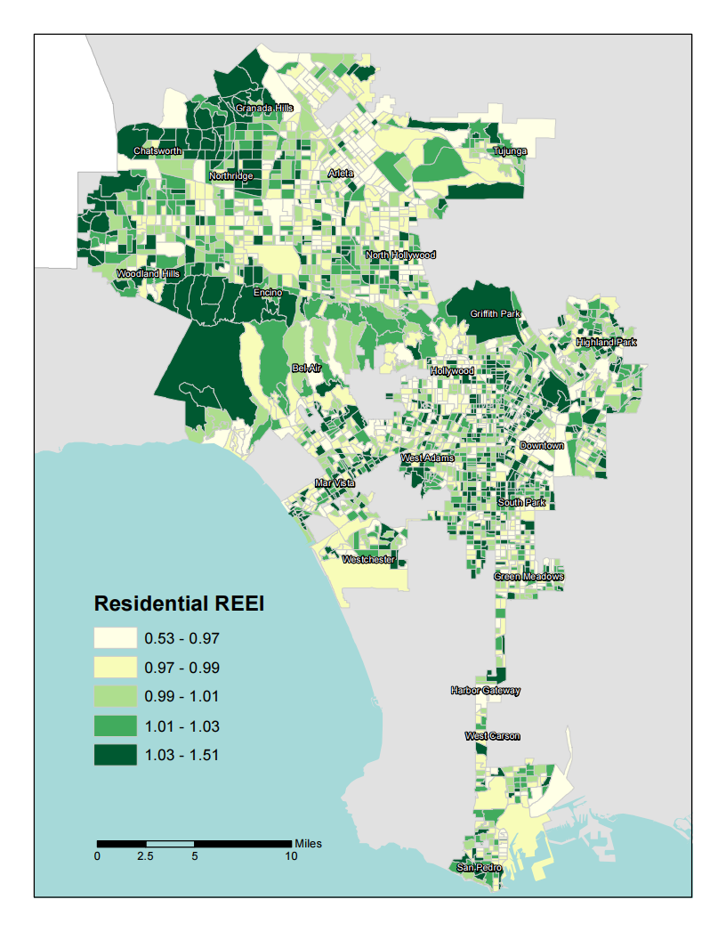
| + | [[File:Map 4.1 Residential Relative Energy Efficiency Index (REEI) 2009-2012.png|200px|framed|center|Residential Relative Energy Efficiency Index (REEI) 2009-2012 Choropleth]] | ||
| + | [[File:Map 4.2 Local Moran's I for Residential REEI.png|200px|framed|center|Local Moran's I for REEI - most and least efficient block groups]] | ||
<br/> | <br/> | ||
| − | |||
<strong>Methodology:</strong><br/> | <strong>Methodology:</strong><br/> | ||
| − | 1. | + | 1. Creation of a REEI (Relative Energy Efficiency Index) |
| − | * | + | * Done by dividing the zonal average consumption growth rate by the consumption change rate for each block group. |
| − | 2. | + | 2. Global Moran’s I |
| − | * | + | * Determine if spatial autocorrelation is taking place |
| + | 3. Local Moran's I | ||
| + | * See where clustering is taking place | ||
<br/> | <br/> | ||
<strong>Learning Points:</strong><br/> | <strong>Learning Points:</strong><br/> | ||
| − | + | 1. REEI (Relative Energy Efficiency Index) | |
| − | 1. | + | * Team can look into calculating such an index for each HDB parcel |
| − | |||
| − | * | ||
| − | |||
| − | |||
<br/> | <br/> | ||
<strong>Areas for improvement:</strong><br/> | <strong>Areas for improvement:</strong><br/> | ||
| − | 1. | + | 1. The temperature data used was too simple - only two zones of temperature. |
| − | * | + | * Our team will use the previously learnt RST interpolation method to create a model for temperature geospatial variation, that also allows for temporal analysis. |
<br/><br/> | <br/><br/> | ||
| − | |||
| − | |||
== Approach == | == Approach == | ||
| − | + | <div style="text-align: left; direction: ltr; margin-left: 1em;"> | |
| − | <br/> | + | <Strong>Data Collection and Preprocessing</Strong> |
| − | + | <p> | |
| − | + | *We collected 2013- 2016 average monthly household electricity consumption by postal code and dwelling type from Energy Market Authority. The postal codes are matched with longitudes and latitudes with the use of OneMap API. | |
| − | + | *Singapore Temperature Historical Data from 2013 to 2016 at daily granularity were crawled from Meteorological Service Singapore. | |
| + | <br> | ||
| + | <Strong>Methodology</Strong> | ||
| + | *Hot Spot and Cold Spot maps: | ||
| + | The maps show which areas have high energy consumption and low energy consumption. First we used adaptive distance weight matrix to define neighbours. Based on the adaptive distance weight matrix, we computed Getis -Ord Gi statistics. A hot spot area has significantly positive Gi statistics which means location i is associated with relatively high values of the surrounding locations. A cold spot area has significantly negative Gi statistics which means location i is associated with relatively low values of the surrounding locations. | ||
| + | *LISA Map | ||
| + | Local Indicator of Spatial Association (LISA) maps help us identify the outliers and clusters of the energy consumption observations. | ||
| − | + | *Spatial Interpolation | |
| − | + | Since we only have 21 meteorological stations that have complete data in Singapore, Spatial interpolation is adopted to use points with known temperature values to estimate values at other unknown points. | |
| − | |||
| − | The | + | *Geographically Weighted Regression Local R square. |
| − | + | The estimated temperature and energy consumption data will be used in the Geographically Weighted Regression (GWR) model. The GWR model will generate Local R square values which indicate how well the local regression model fits observed y values. Very low values indicate the local model is performing poorly. In our case, it means low correlation between temperature and energy in the areas. | |
| − | |||
| − | |||
| − | |||
| − | |||
| − | |||
| − | |||
| − | |||
| − | |||
| − | |||
| − | |||
| − | |||
| − | |||
| − | |||
| − | |||
| − | |||
| − | |||
| − | |||
| − | |||
| + | </div> | ||
| − | |||
== Web Application Design == | == Web Application Design == | ||
=== Design Inspiration === | === Design Inspiration === | ||
| + | The dashboard design is inspired by https://stanleyadion.shinyapps.io/AmazeingCrop | ||
<br/> | <br/> | ||
| − | |||
| − | |||
| − | |||
| − | |||
| − | |||
| − | |||
=== Initial Storyboard === | === Initial Storyboard === | ||
| − | |||
| − | |||
| − | |||
| − | |||
| − | |||
| − | |||
| − | |||
| − | |||
| − | |||
| − | |||
| − | |||
| − | |||
| − | |||
| − | |||
{| class="wikitable" | {| class="wikitable" | ||
|- | |- | ||
| − | ! | + | ! !! Design !! Description |
|- | |- | ||
| − | | | + | | 1. ||[[File:Elec3city dashboard 1.jpg|600 px]] || |
| − | * | + | * Project and Dataset Overview |
| − | |||
| − | |||
|- | |- | ||
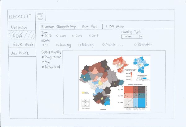
| − | | | + | | 2. ||[[File:Elec3city dashboard 2.jpg|600 px]] || |
| − | * | + | * Bivariate Choropleth Maps showing relationships between energy consumption with other factors |
| + | * Users can choose the factor they want to compare with energy consumtion | ||
|- | |- | ||
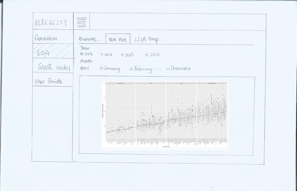
| − | | | + | | 3. ||[[File:Elec3city dashboard 3.jpg|600 px]] || |
| − | * | + | * A Box-plot showing distributions of energy consumption by Planning Zone and Dwelling Type |
|- | |- | ||
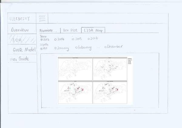
| − | | | + | | 4. ||[[File:Elec3city dashboard 4.jpg|600 px]] || |
| − | * | + | * Lisa Maps showing spatial clustering of energy consumption observations |
|- | |- | ||
| − | | | + | | 5. ||[[File:Elec3city dashboard 5.jpg|600 px]] || |
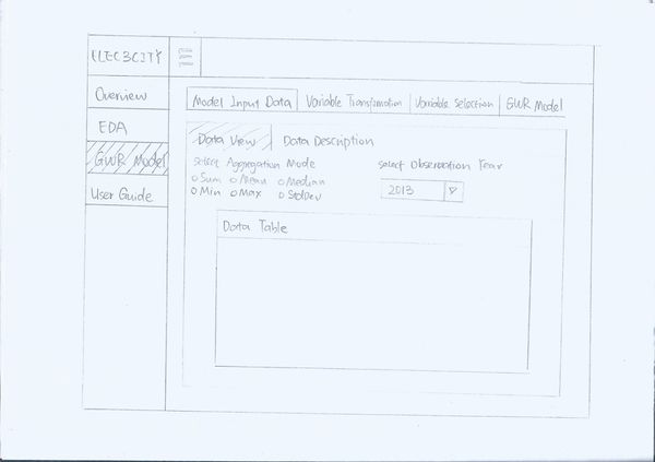
| − | * | + | * Overview of Data for GWR model |
| − | |||
| − | |||
| − | |||
| − | |||
| − | |||
| − | |||
| − | |||
| − | |||
|- | |- | ||
| − | | | + | | 6. ||[[File:Elec3city dashboard 6.jpg|600 px]] || |
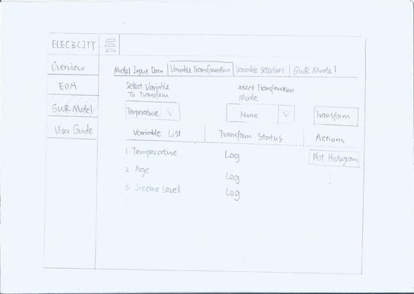
| − | * | + | * Transform Data for GWR model |
| − | * | + | * Users can use a histogram to check whether the variable is normally distributed |
| − | |||
|- | |- | ||
| − | | | + | | 7. ||[[File:Elec3city dashboard 7.jpg|600 px]] || |
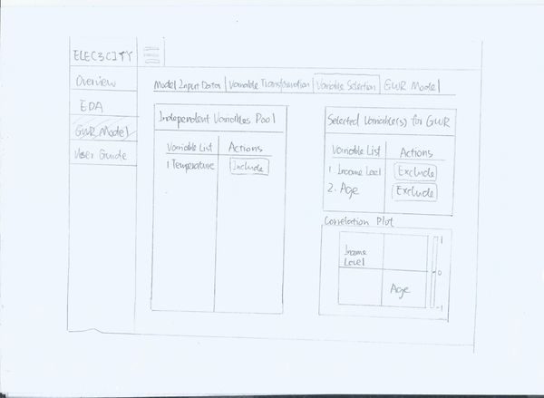
| − | * | + | * Select Variables for GWR model |
| + | * Users can remove correlated variables with the help of the correlation matrix plot | ||
|- | |- | ||
| − | | | + | | 8. ||[[File:Elec3city dashboard 8.jpg|600 px]] || |
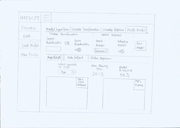
| − | * | + | * Configure a GWR model and view the results |
| − | |||
| − | |||
| − | |||
| − | |||
| − | |||
| − | |||
| − | |||
| − | |||
| − | |||
| − | |||
| − | |||
| − | |||
| − | |||
| − | |||
| − | |||
| − | |||
| − | |||
| − | |||
|} | |} | ||
| − | |||
| − | |||
| − | |||
| − | |||
| − | |||
| − | |||
| − | |||
| − | |||
| − | |||
| − | |||
| − | |||
| − | |||
| − | |||
| − | |||
| − | |||
| − | |||
| − | |||
| − | |||
| − | |||
| − | |||
| − | |||
| − | |||
| − | |||
| − | |||
| − | |||
| − | |||
| − | |||
| − | |||
| − | |||
| − | |||
| − | |||
| − | |||
| − | |||
| − | |||
== Project Challenges == | == Project Challenges == | ||
{| class="wikitable" | {| class="wikitable" | ||
| Line 383: | Line 246: | ||
! !! Key Challenges !! Description !! Solution | ! !! Key Challenges !! Description !! Solution | ||
|- | |- | ||
| − | | 1. || | + | | 1. ||Temperature Data Collection ||We can only download the temperature data from Meteorological Service Singapore for one station and one month each time. There are more than 60 stations and 4 years of data to be downloaded for this project, which can be very time consuming. || |
| − | * | + | * Discovered a pattern of the data links |
| − | * | + | * Used excel to auto-generate all the required data links |
| + | * Used Internet Download Manager to download from all the data links | ||
|- | |- | ||
| − | | 2. || | + | | 2. ||Imperfect Temperature Data ||Temperature information is only collected at the designated temperature stations. || |
| − | * | + | * Use spatial interpolation techniques to estimate the temperature around the temperature stations. |
| − | + | ||
| − | |||
| − | |||
| − | |||
| − | |||
| − | |||
| − | |||
| − | |||
| − | |||
|} | |} | ||
<br/><br/> | <br/><br/> | ||
<br/> | <br/> | ||
| + | |||
== Project Timeline == | == Project Timeline == | ||
| − | + | ||
<br/><br/> | <br/><br/> | ||
| − | + | [https://docs.google.com/spreadsheets/d/1uUxaRZqa5FhF3voPMc0w3HcNnOHgbFlnvJWyN4htZPE/edit#gid=734092126 Gantt Chart of Team's Timeline - FULL Updated Version]<br> | |
| − | + | Snapshot of Gantt Chart (as of 3 March 2019) | |
| − | + | [[File:Gantt Chart2.png|left|1000px|Gantt Chart Snapshot]]<br><br><br><br><br><br><br><br><br><br><br><br><br><br><br><br><br><br><br><br><br><br><br><br><br><br><br><br><br> | |
| − | [[File: | ||
| − | < | ||
| − | <br> | ||
| − | |||
| − | |||
<div style="text-align: center; direction: ltr; margin-left: 1em;"><font face="Avenir"><big>Feel free to leave any comments! :) </big></font></div> | <div style="text-align: center; direction: ltr; margin-left: 1em;"><font face="Avenir"><big>Feel free to leave any comments! :) </big></font></div> | ||
Latest revision as of 19:04, 14 April 2019
Contents
Project Motivation
Rising energy consumption is an issue that plagues the Singapore government for several years. Recently, the government has begun pushing for more efficient energy usage, and most effort is expended on the efficiency of energy sources – e.g. using less carbon-intensive fuels. In exploring potential ways to aid this cause, we realised that there has been scant statistical analysis energy consumption patterns. As such, our team feels that there is a need for an app which allows for authorities in Singapore such as the National Environment Agency to understand with data-driven evidence the origins of variation in Singapore energy consumption, so as to allow for more targeted efforts to reduce energy wastage. Another factor that provided a fertile ground for the development of this application is the availability of energy consumption data, with granularity right down to individual postal code.
Project Objective
We have been observing rising trends in energy consumption across all sub-sectors, including households, which has seen sharp increase over the years from 6092.5GWh in 2005 to 7295.8GWh in 2017. As such, household sub-sector is a good starting point for our analysis.
- Energy Consumption Patterns in Singapore
Through the exploration of potential energy consumption patterns among households in Singapore, we will be able to tease out potential drivers of energy consumption. We will not only be looking at seasonal patterns in consumption (i.e. Is there a particular month in a year when energy consumption spikes?), we will also try to identify spatial patterns in consumption (i.e. Is there a particular region in Singapore whereby energy consumption is particularly high?).
- Temperature VS Energy Consumption
The next issue that we are interested in exploring is the relationship between temperature and energy consumption. Intuitively, we will assume that as temperature increases, energy consumption will also increase due to more electrical appliances used to regulate temperature such as air-conditioner. Thus, we plan to explore the relationship between temperature in different region of Singapore, and how this will affect the energy consumption in each respective region.
Data
Literature Review
In our due diligence for the project, the team looked at multiple research papers to inform and influence us in the best practices for analyzing geospatial variation in energy use, when it is to be compared against variables such as temperature and housing composition.
1. Appropriate use of Interpolation Methods in GIS - Mitas, L. and Mitasova, H. Spatial Interpolation, Chap. 34 Spatial Interpolation (2005)Aim of literature: to enlighten reader of the appropriate interpolation method for different GIS themes.
Methodology:
1. Inverse Distance Weighted Interpolation (IDW) - adopted
2. Kriging - rejected
3. Regularised spline with tension (RST) - rejected
Learning Points:
1. Inverse Distance Weighted Interpolation (IDW)
- Pro: relatively less demanding computationally
- Pro: better at reproducing approximations on linear patterns
- Con: "produces local extrema at the data points"
2. Kriging
- Con: While good at predicting spatial distribution of uncertainty, it is less successful for applications where local geometry and smoothness are the key issues - Critical weakness for our interpolation of temperature data where granularity is at housing block level, thus Kriging is rejected.
3. Regularised spline with tension (RST)
- Pro: Allows for smoothing according to parameters such as the tension φ and smoothing weights {wj} which are empirically informed through minimisation of the predictive error estimated by a cross-validation procedure
- Pro: Can realistically represent rough gradients in spite of the smoothness condition, if the roughness is sufficiently described by the input data - might be true of temperature when it comes to the Urban Heat Island effect - pockets of high building density can cause a micro-climate of higher temperatures; particularly pertinent in Singapore.
- Con: requires a lot of 'guess-timation' and past domain knowledge to fine-tune the tension and smoothing weights.
Areas for improvement:
Our team has selected IDW as the interpolation technique for smoothing of temperature data of the 22 weather stations across Singapore.
Aim of literature: investigate poverty and inequities that are associated with vegetation
Methodology:
1. Pixel level regression - Curve Fit extension in ArcGIS
- Run regression trend analysis using raster datasets for temporal analysis
2. Global Ordinary Least Squares (OLS) regression
- Capture global geospatial correlation
3. Local Geographically Weighted Regression (GWR)
- Capture local geospatial correlation
4. Moran's I for spatial autocorrelation
- For local level analysis of spatial autocorrelation
5. Local Indicators of Spatial Association (LISA) map - Contiguity Edges and Corners method
- Queen contiguity to show clustering
Learning Points:
1. Pixel level regression - Curve Fit extension in ArcGIS
- Helps us see the degree of model prediction for energy consumption given our variables
2. Global Ordinary Least Squares (OLS) regression
- Investigate if the distributions of these random variables all have the same variance and a mean of zero. If so, then the least squares method may be the best unbiased linear estimator of the model coefficient.
- If residuals are spatially correlated, OLS results are biased. GWR models would then be used to remove the spatial autocorrelation of residuals.
3. Local Geographically Weighted Regression (GWR)
- Provides local t-values with which to find level of confidence in our local model
4. Moran's I for spatial autocorrelation
- We can use this to ascertain if local level analysis is indeed appropriate to understand the relationship between income level and energy consumption, after accounting for other factors like number of household members and number of rooms.
5. Local Indicators of Spatial Association (LISA) map - Contiguity Edges and Corners method
- Shows us clustering of energy consumption at local level
Areas for improvement:
1. Pixel level regression - Curve Fit extension in ArcGIS
- No ArcGIS - so we use curveFit function provided in mixtox v1.3 package by Xiangwei Zhu
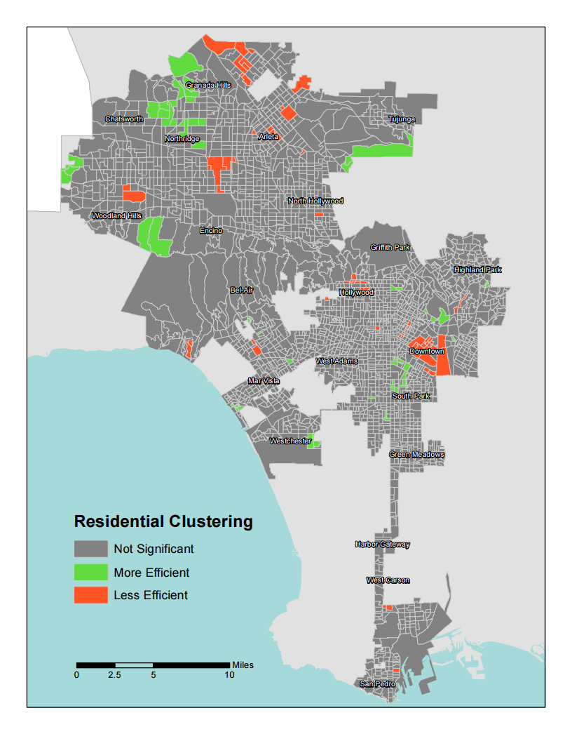
Aim of literature: reduce traditional energy usage and promoting sustainable energy production through geographically segmented marketing
Methodology:
1. Creation of a REEI (Relative Energy Efficiency Index)
- Done by dividing the zonal average consumption growth rate by the consumption change rate for each block group.
2. Global Moran’s I
- Determine if spatial autocorrelation is taking place
3. Local Moran's I
- See where clustering is taking place
Learning Points:
1. REEI (Relative Energy Efficiency Index)
- Team can look into calculating such an index for each HDB parcel
Areas for improvement:
1. The temperature data used was too simple - only two zones of temperature.
- Our team will use the previously learnt RST interpolation method to create a model for temperature geospatial variation, that also allows for temporal analysis.
Approach
Data Collection and Preprocessing
- We collected 2013- 2016 average monthly household electricity consumption by postal code and dwelling type from Energy Market Authority. The postal codes are matched with longitudes and latitudes with the use of OneMap API.
- Singapore Temperature Historical Data from 2013 to 2016 at daily granularity were crawled from Meteorological Service Singapore.
Methodology
- Hot Spot and Cold Spot maps:
- LISA Map
- Spatial Interpolation
- Geographically Weighted Regression Local R square.
Web Application Design
Design Inspiration
The dashboard design is inspired by https://stanleyadion.shinyapps.io/AmazeingCrop
Initial Storyboard
Project Challenges
| Key Challenges | Description | Solution | |
|---|---|---|---|
| 1. | Temperature Data Collection | We can only download the temperature data from Meteorological Service Singapore for one station and one month each time. There are more than 60 stations and 4 years of data to be downloaded for this project, which can be very time consuming. |
|
| 2. | Imperfect Temperature Data | Temperature information is only collected at the designated temperature stations. |
|
Project Timeline
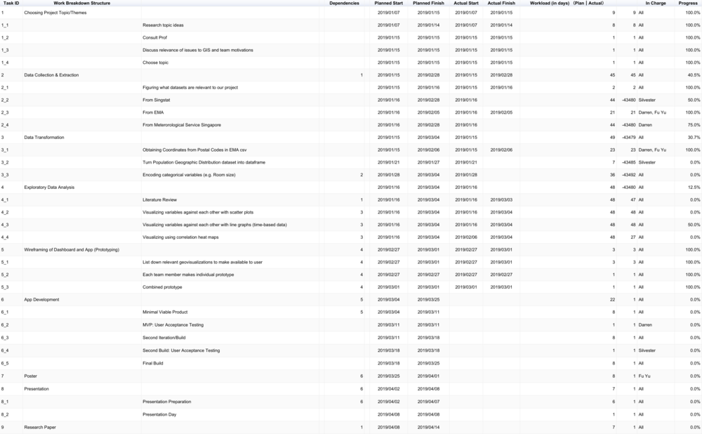
Gantt Chart of Team's Timeline - FULL Updated Version
Snapshot of Gantt Chart (as of 3 March 2019)
|
No. |
Name |
Date |
Comments |
|
1. |
Insert your Name here |
Insert Date here |
Insert Comment here |
|
2. |
Insert your Name here |
Insert Date here |
Insert Comment here |
|
3. |
Insert your Name here |
Insert Date here |
Insert Comment here |
