Difference between revisions of "Signal Proposal"
Mechong.2015 (talk | contribs) |
Mechong.2015 (talk | contribs) |
||
| (109 intermediate revisions by 2 users not shown) | |||
| Line 19: | Line 19: | ||
| style="font-family:Open Sans, Arial, sans-serif; font-size:15px; text-align: center; border-top:solid #ffffff; border-bottom:solid #f5f5f5" width="230px" | | | style="font-family:Open Sans, Arial, sans-serif; font-size:15px; text-align: center; border-top:solid #ffffff; border-bottom:solid #f5f5f5" width="230px" | | ||
[[Signal_Research_Paper|<font color="#3c3c3c"><strong>RESEARCH PAPER</strong></font>]] | [[Signal_Research_Paper|<font color="#3c3c3c"><strong>RESEARCH PAPER</strong></font>]] | ||
| + | |||
| + | | style="font-family:Open Sans, Arial, sans-serif; font-size:15px; text-align: center; border-top:solid #ffffff; border-bottom:solid #f5f5f5" width="230px" | | ||
| + | [[Project_Groups|<font color="#3c3c3c"><strong>RETURN TO PROJECT GROUPS</strong></font>]] | ||
|} | |} | ||
| Line 28: | Line 31: | ||
==<div style="background:#143c67; padding: 15px; font-weight: bold; line-height: 0.3em; letter-spacing:0.5em;font-size:20px"><font color=#fbfcfd face="Lato"><center>PROBLEM & MOTIVATION</center></font></div>== | ==<div style="background:#143c67; padding: 15px; font-weight: bold; line-height: 0.3em; letter-spacing:0.5em;font-size:20px"><font color=#fbfcfd face="Lato"><center>PROBLEM & MOTIVATION</center></font></div>== | ||
| − | + | In order to attempt to reduce traffic accidents, it is important to understand where, when and who is involved in traffic accidents. A better understanding of spatio-temporal patterns specific to casualty groups aids in developing appropriate preventive measures by the authorities. For example, a road segment could have high intensity of traffic accidents for the elderly but those traffic accidents could possibly occur only at certain time periods, such as at night. | |
| − | + | In view of the benefits of applying spatio-temporal analyses to traffic accidents, our initial focus was on developing a web-based geospatial application for Singapore as there is a general lack of spatio-temporal geospatial applications developed specific to this area. Most web-enabled geospatial application tools are also limited to analysing non-network constrained accident point patterns. The Singapore Police Force is also concerned about accidents involving motorcyclists and elderly jaywalkers as motorcyclist accidents still account for more than half of the traffic accidents in 2017, and the number of elderly road fatalities have been on the rise (Chua, 2018). | |
| − | + | Although this serves as grounds for adapting our application to Singapore’s context, our team has used data from Leeds, United Kingdom instead, due to its easily accessible rich diversity of information. Specifically, Leeds’ traffic accident data includes coordinates of traffic accidents, time, weather and details on casualties, all of which are essential for an in-depth spatio-temporal analysis for a certain casualty group. While behavioral patterns of drivers and pedestrians in United Kingdom may not be reflective of that of Singapore’s, insights still provides some indicative directions for investigations by Singapore Land Transport Authority and Singapore Police Force. | |
| − | + | ||
| + | As such, a web-enabled geospatial analytics tool, SIGNAL, was developed with the purpose of allowing users to conduct network-constrained statistical analyses on road networks for selected target groups or environmental conditions. | ||
==<div style="background:#143c67; padding: 15px; font-weight: bold; line-height: 0.3em;letter-spacing:0.5em;font-size:20px"><font color=#fbfcfd face="Lato"><center>OBJECTIVES</center></font></div>== | ==<div style="background:#143c67; padding: 15px; font-weight: bold; line-height: 0.3em;letter-spacing:0.5em;font-size:20px"><font color=#fbfcfd face="Lato"><center>OBJECTIVES</center></font></div>== | ||
| − | In our project, we would be creating | + | In our project, we would be creating an analytical tool for discovering network-constrained spatio-temporal patterns of traffic accidents. Specifically, it focuses on the following objectives: |
| − | * | + | *To visualise the intensity of traffic accidents on road networks cartographically on an internet-based map such as Esri |
| − | + | *To conduct statistical simulations on road segments to reveal evidence of clusters or correlation patterns | |
| − | * | + | *To provide a user-friendly interface to for practitioners to apply relevant filters for different time periods selected |
| − | * | ||
==<div style="background:#143c67; padding: 15px; font-weight: bold; line-height: 0.3em;letter-spacing:0.5em;font-size:20px"><font color=#fbfcfd face="Lato"><center>SELECTED DATASETS</center></font></div>== | ==<div style="background:#143c67; padding: 15px; font-weight: bold; line-height: 0.3em;letter-spacing:0.5em;font-size:20px"><font color=#fbfcfd face="Lato"><center>SELECTED DATASETS</center></font></div>== | ||
| Line 51: | Line 54: | ||
!| Source | !| Source | ||
|- | |- | ||
| − | | Leeds Road Traffic Accidents ( | + | | Leeds Road Traffic Accidents (2013 - 2017) |
| CSV | | CSV | ||
| | | | ||
| Line 70: | Line 73: | ||
* Age of Casualty | * Age of Casualty | ||
| [https://data.gov.uk/dataset/6efe5505-941f-45bf-b576-4c1e09b579a1/road-traffic-accidents UK Open Database] | | [https://data.gov.uk/dataset/6efe5505-941f-45bf-b576-4c1e09b579a1/road-traffic-accidents UK Open Database] | ||
| + | |- | ||
| + | | Leeds Pedestrian Crossing | ||
| + | | CSV | ||
| + | | | ||
| + | * Installation_Type | ||
| + | * ORN | ||
| + | * Address | ||
| + | * Easting | ||
| + | * Northing | ||
| + | * Postal Code | ||
| + | | [https://datamillnorth.org/dataset/pedestrian-crossing-points Leeds Council Data Mill North] | ||
| + | |- | ||
| + | | Leeds School | ||
| + | | CSV | ||
| + | | | ||
| + | * DfE | ||
| + | * DfE_Old | ||
| + | * URN | ||
| + | * URN_Old | ||
| + | * School | ||
| + | * Phase | ||
| + | * TypeDetail | ||
| + | * ReligiousCharacter | ||
| + | * Years | ||
| + | * Postcode | ||
| + | * X REF | ||
| + | * Y REF | ||
| + | * Ward_new | ||
| + | * Constituency | ||
| + | *lsoa01 | ||
| + | *lsoa11 | ||
| + | *ClusterThisYear | ||
| + | *OpenOrClosed | ||
| + | | [https://data.gov.uk/dataset/862490b9-7771-4bac-8152-c435d7602232/leeds-schools UK Open Database] | ||
|- | |- | ||
| Local Authority Districts (Leeds) | | Local Authority Districts (Leeds) | ||
| Line 77: | Line 114: | ||
|- | |- | ||
| Leeds Road | | Leeds Road | ||
| − | |||
| − | |||
| − | |||
| − | |||
| − | |||
| SHP | | SHP | ||
| | | | ||
| Line 93: | Line 125: | ||
|} | |} | ||
<br> | <br> | ||
| + | |||
==<div style="background:#143c67; padding: 15px; font-weight: bold; line-height: 0.3em;letter-spacing:0.5em;font-size:20px"><font color=#fbfcfd face="Lato"><center>DATA PREPARATION</center></font></div>== | ==<div style="background:#143c67; padding: 15px; font-weight: bold; line-height: 0.3em;letter-spacing:0.5em;font-size:20px"><font color=#fbfcfd face="Lato"><center>DATA PREPARATION</center></font></div>== | ||
| + | [[File:Flow.png|800px|frameless|center]] | ||
| + | <b>Data Collection</b><br> | ||
| + | Data of Leeds Traffic Accident Data (2013 to 2017), Schools and Pedestrian Crossings data were collected from the UK Open Database in CSV file format, while Leeds’ District Boundary Map, Road Network and Motorway Junctions were obtained from UK Consumer Data Research Centre (CDRC) in Shapefile (SHP) format. | ||
| + | <br> | ||
| − | + | <b>Data Cleaning and Wrangling</b><br> | |
| + | Traffic accident point events were separated from casualty point events before removing duplicates. Unique accident points allow for visualization of intensity and spatial distribution of traffic accidents. Standardization of data, such as, ensuring columns of each CSV files and their data types are the same before reclassifying selected columns, is conducted. | ||
| + | <br> | ||
| + | [[File:Photo 2019-04-15 00-57-18.jpg|600px|frameless|center]] | ||
| + | <b>Data Transformation</b><br> | ||
| + | As our geospatial application involves the use of Network Constrained analyses, data has to be transformed to appropriate formats before relevant functions could be used. Specifically, accident traffic points have to be converted to SpatialPoints and then to Point Pattern Processes. Roads would have to be converted to SpatialLines and then to Linnet before they could be combined with Point Patterns Processes to form Linear Point Patterns. In order to constrain the Linear Point Patterns to a target area of interest, it has to be intersected with the Owin of District Boundary Map. The below figure summarises the key data transformation that takes place. | ||
==<div style="background:#143c67; padding:15px; font-weight: bold; line-height: 0.3em;letter-spacing:0.5em;font-size:20px"><font color=#fbfcfd face="Lato"><center>LITERATURE REVIEW</center></font></div>== | ==<div style="background:#143c67; padding:15px; font-weight: bold; line-height: 0.3em;letter-spacing:0.5em;font-size:20px"><font color=#fbfcfd face="Lato"><center>LITERATURE REVIEW</center></font></div>== | ||
| Line 140: | Line 182: | ||
=== 3. Analysis of data on the dataset of road accidents in Paris in 2012 and 2013 === | === 3. Analysis of data on the dataset of road accidents in Paris in 2012 and 2013 === | ||
| + | http://www.remyzum.com/shiny/Paris_Accidentologie/ | ||
''(By: Remy Zumbiehl)'' | ''(By: Remy Zumbiehl)'' | ||
| Line 147: | Line 190: | ||
<b>Methodology</b>: | <b>Methodology</b>: | ||
| − | # | + | # Basic Mapping using Leaflet Package |
| − | |||
| − | |||
| − | |||
| − | |||
| − | |||
<b>Learning Points</b>: | <b>Learning Points</b>: | ||
| Line 162: | Line 200: | ||
<b>Areas for Improvement</b>: | <b>Areas for Improvement</b>: | ||
* Add in geospatial analysis such as Kernel Density Estimation and Network Constrained Analysis | * Add in geospatial analysis such as Kernel Density Estimation and Network Constrained Analysis | ||
| − | |||
<br> | <br> | ||
==<div style="background:#143c67; padding:15px; font-weight: bold; line-height: 0.3em;letter-spacing:0.5em;font-size:20px"><font color=#fbfcfd face="Lato"><center>APPROACH</center></font></div>== | ==<div style="background:#143c67; padding:15px; font-weight: bold; line-height: 0.3em;letter-spacing:0.5em;font-size:20px"><font color=#fbfcfd face="Lato"><center>APPROACH</center></font></div>== | ||
| − | + | After analysing several literature reviews, it is clearly inappropriate to use the standard point pattern analysis used for two-dimensional space. Our analyses need to take into account the geometry of the network and as such, we have to constrain statistical techniques such as K-Function to the network. We will first delve into uncovering which road segments have a higher intensity of road accidents followed by using various network-constrained techniques to investigate if there are statistically significant clusters. | |
| + | |||
| + | ===1. Network Constrained Kernel Density Estimation=== | ||
| + | |||
| + | Kernel Density Estimation involves estimating the probability density function of a variable, or in other words the density of features in a neighbourhood in geospatial terms. Investigating the average density of points along the network provides a quick insight on which segments of roads has higher intensity of traffic accidents. | ||
| + | |||
| + | There are two main types of intensities when estimating kernel densities in networks: | ||
| + | |||
| + | * Homogeneous intensity function has randomness that is characterised by complete spatial randomness. All points are independent and uniformly distributed in any given set. | ||
| + | * Inhomogeneous intensity function also has independence between disjoint sets but points are unevenly distributed according to their spatially varying intensity functions. | ||
| + | |||
| + | Homogeneous intensity is used as traffic accidents are assumed to occur in spatial randomness. The kernel estimate of intensity has the form: | ||
| + | |||
| + | [[File:Inhomogeneous Intensity.png|200px|frameless|center]] | ||
| + | |||
| + | k(v,u) is the smoothing kernel to smooth out a point on the network, as shown below, in a book by Adrian et al (2016). The smoothing of the point is done with a Gaussian kernel and thickness of line proportional to the kernel value. This can be performed using the density.lpp function in R. | ||
| + | |||
| + | [[File:Smoothing.png|400px|frameless|center]] | ||
| + | |||
| + | ===2. Second-Order Network Constrained K-Function (Network Constrained Ripley's K-Function)=== | ||
| + | |||
| + | After gaining insight on the density of traffic accidents, we would take the next step to uncover if the point patterns are dispersed, clustered or randomly distributed. This could be done using Network K-Function. | ||
| + | |||
| + | The Okabe-Yamada network K-Function defines the Network K-Function, by adapting the Ripley’s K Function through replacing the Euclidean distance with the shortest path distance. In this method, given a point v on the network, all locations in the network that can be reached from v by a path of length shorter than a radius r, defined by the user, would be considered. It is defined by the function below, with lambda(L) denoting the total length of the linear network : | ||
| + | |||
| + | [[File:Okabe Network K.png|400px|frameless|center]] | ||
| + | |||
| + | While the above Network K-Function constrains points to networks, a second-order stationary point process is required for our analyses. The Okabe-Yamada network K-Function assumes that the network itself is homogeneous, which is not the case as different locations in the network is surrounded by different configurations of line segments. Network K-Functions obtained from different networks are not directly compatible in this case. | ||
| + | |||
| + | The second-order Network K-Function is proposed by Ang et al (2012) , known as the ‘geometrically corrected K-Function’. It is an extension of the Ripley’s K-Function’s benefits of enabling comparison between different point processes with different intensities, observed in different windows, combined with Okabe-Yamada network K-function. The geometrically corrected K-Function is defined by, for all r ≤ R, where u is any location on the network: | ||
| + | |||
| + | [[File:GC K-Function.png|400px|frameless|center]] | ||
| + | |||
| + | The above analysis can be computed in spatstat by the function linearK. It is noted that K-Function assumes homogeneity. | ||
| + | |||
| + | ===3. Correlation in Multitype Point Patterns Using Network Constrained Cross K-Function=== | ||
| + | |||
| + | Network Constrained K-Function handles points of the same type while Network Constrained Cross-K Function is used for two different sets of points. Estimation is based on measuring pairwise distances from all points of type i to all points of type j. Thus, for any pair of types i and j, the function calculates the expected number of points of type j lying within a distance r of a typical point of type i, standardised by dividing the intensity of points of type j, for r >= 0. The Cross-K Function is as shown below and it is constrained to a network in our application. | ||
| + | |||
| + | [[File:Screenshot 2019-04-14 at 11.43.14 PM.png|300px|frameless|center]] | ||
| + | |||
| + | This can be implemented in R through the function linearKcross. | ||
<br> | <br> | ||
| + | |||
| + | ===4. Correlation in Multitype Point Patterns Using Network Constrained Cross Pair Correlation=== | ||
| + | Similar to Network Constrained Cross K-Function, Network Constrained Cross Pair Correlation Function measures pairwise distances from all points of type i to all points of type j. However, this function calculates the expected number of points of type j lying at a distance equal to distance r of a typical point of type i, standardised by dividing the intensity of points of type j, for r >= 0. The cross pair correlation function is as shown below, and it is constrained to a network in our application. | ||
| + | |||
| + | [[File:Screenshot 2019-04-15 at 12.17.48 AM.png|300px|frameless|center]] | ||
| + | |||
| + | This analysis is computed in spatstat by the function linearpcfcross. | ||
==<div style="background:#143c67; padding:15px; font-weight: bold; line-height: 0.3em;letter-spacing:0.5em;font-size:20px"><font color=#fbfcfd face="Lato"><center>STORYBOARD</center></font></div>== | ==<div style="background:#143c67; padding:15px; font-weight: bold; line-height: 0.3em;letter-spacing:0.5em;font-size:20px"><font color=#fbfcfd face="Lato"><center>STORYBOARD</center></font></div>== | ||
| − | [[File: | + | After rounds of refinement, below are the storyboard of our application: </br> |
| + | <b>Network Constrained KDE page</b> | ||
| + | [[File:Slide11.png|800px|frameless|center]] | ||
| + | Network Constrained KDE page will have 2 maps to show traffic accidents and casualty KDE to allow the user to compare the map. Filters and a kernel distance slider will be at the right-hand side of the application. | ||
| + | <br><br> | ||
| + | <b>Network Constrained K-Function page</b> | ||
| + | [[File:Slide22.png|800px|frameless|center]] | ||
| + | Network Constrained K-Function page will have a map at the top and a result box at the bottom which consists of the analysis graph output along with the interpretation function of the graph. Filters and simulation slider will be at the right-hand side of the application. | ||
| + | <br><br> | ||
| + | <b>Network Constrained Cross K-Function and Network Constrained Cross Pair Correlation Function page</b> | ||
| + | [[File:Slide33.png|800px|frameless|center]] | ||
| + | Network Constrained Cross K-Function and Network Constrained Cross Pair Correlation Function page will have a map at the top and a result box at the bottom which consists of the analysis graph output along with the interpretation function of the graph. Filters, a variable selection dropdown bar and simulation slider will be at the right-hand side of the application. | ||
==<div style="background:#143c67; padding:15px; font-weight: bold; line-height: 0.3em;letter-spacing:0.5em;font-size:20px"><font color=#fbfcfd face="Lato"><center>TOOLS & TECHNOLOGIES</center></font></div>== | ==<div style="background:#143c67; padding:15px; font-weight: bold; line-height: 0.3em;letter-spacing:0.5em;font-size:20px"><font color=#fbfcfd face="Lato"><center>TOOLS & TECHNOLOGIES</center></font></div>== | ||
<b>Tools and technologies</b> | <b>Tools and technologies</b> | ||
<br/> | <br/> | ||
| − | + | [[File:Tools signal.png|600px|frameless|center]] | |
<br/> | <br/> | ||
<b>Data Architecture</b> | <b>Data Architecture</b> | ||
<br/> | <br/> | ||
| − | [[File:Architecture.png|frameless|center| | + | [[File:Architecture.png|frameless|center|600px]] |
<br/> | <br/> | ||
| + | |||
| + | ==<div style="background:#143c67; padding: 15px; font-weight: bold; line-height: 0.3em; letter-spacing:0.5em;font-size:20px"><font color=#fbfcfd face="Lato"><center>APPLICATION OVERVIEW</center></font></div>== | ||
| + | <b>Network Constrained Kernel Density Estimation</b> | ||
| + | [[File:Kde 2.png|800px|frameless|center]] | ||
| + | <br> | ||
| + | <b> Other Network Constrained Analysis </b></br> | ||
| + | Network Constrained K-Function, Network Constrained Cross K-Function and Network Constrained Cross Pair Correlation Function have the same layout. | ||
| + | [[File:Function.png|800px|frameless|center]] | ||
| + | {| class="wikitable" width="100%" | ||
| + | |- | ||
| + | ! style = "width: 30%;" | Component | ||
| + | ! style="width: 70%;"| Purpose | ||
| + | |- | ||
| + | | <b>Leeds Map</b></br> | ||
| + | [[File:Map.png|400px|frameless|left]] | ||
| + | | The markers are to indicate the geographical positions of traffic accidents and other variables (Pedestrian Crossing, Motorway Junctions and Schools). The user is able to zoom in and move the map using the map control button to an area that they wish to run the analysis on. | ||
| + | |- | ||
| + | | <b>Kernel Density Estimation Maps</b></br> | ||
| + | [[File:Kde zoom.png|400px|frameless|left]] | ||
| + | | The user is able to zoom in and move the map using the map control button to an area that they wish to run the analysis on. When the user move or zoom into the top map, the bottom map will be updated automatically as both maps are sync together. This is to ensure that the analysis on both maps are at the same geographical area so that the user is able to have a fair comparison between both maps. | ||
| + | |- | ||
| + | | <b>Time Filters</b></br> | ||
| + | [[File:Time filters.png|150px|frameless|left]] | ||
| + | | The user will be able to filter the data by year, month and hours. | ||
| + | |- | ||
| + | | <b> Environment Filters </b></br> | ||
| + | [[File:Env filters.png|150px|frameless|left]] | ||
| + | | The user will be able to filter the data by: </br> | ||
| + | * <b>Weather conditions </b> – All, Fine without high winds, Fine with high winds, Snowing without high winds, Snowing with high winds, Raining without high winds, Raining with high winds, Fog or mist, unknown and others | ||
| + | * <b>Road Surface</b> – All, Dry, Frost / Ice, Wet / Damp, Snow, Others and Flood (surface water over 3cm deep) | ||
| + | |- | ||
| + | | <b> Casualty Filters </b></br> | ||
| + | [[File:Casualty filters.png|150px|frameless|left]] | ||
| + | | The user will be able to filter the data by: | ||
| + | * <b>Vehicle Class</b> – All, Car, Motorcycle, Bus / Coach, Bicycle, Goods Vehicle, Taxi / Private Hire, Mini Bus, Agricultural Vehicle, Mobility Scooter, Horse and Tram | ||
| + | * <b>Age Group</b> – All, Adult, Elderly, Children and Young Adults | ||
| + | * <b>Type of Casualty</b> – All, Driver or rider, Passenger and Pedestrian | ||
| + | * <b>Casualty Severity</b> – All, Slight, Serious and Fatal | ||
| + | |- | ||
| + | | <b>Kernel Distance Slider</b></br> | ||
| + | [[File:Kernel.png|200px|frameless|left]] | ||
| + | | The bandwidth of kernel density plot. The user is able to drag the slider to state the kernel distance in metre which they want to run for the analysis. | ||
| + | |- | ||
| + | | <b>Simulation Slider</b></br> | ||
| + | [[File:Simulations.png|200px|frameless|left]] | ||
| + | | The user is able to drag the slider to state the number of simulations which they want to run for the analysis. | ||
| + | |- | ||
| + | | <b>Variable Selection</b></br> | ||
| + | [[File:Variable.png|200px|frameless|left]] | ||
| + | | The user is able to choose which variable they want to run the analysis with the traffic accidents. This variable selection is only for Network Constrained Cross K-Function and Network Constrained Cross Pair Correlation Function analysis. | ||
| + | |- | ||
| + | | <b>Network Constrained K-Function</b></br> | ||
| + | [[File:Kfunction.png|400px|frameless|left]] | ||
| + | | Output for Network Constrained K-Function Analysis | ||
| + | |- | ||
| + | | <b>Network Constrained Cross K-Function</b></br> | ||
| + | [[File:Crossk.png|400px|frameless|left]] | ||
| + | | Output for Network Constrained Cross K-Function Analysis | ||
| + | |- | ||
| + | | <b>Network Constrained Cross Pair Correlation Function</b></br> | ||
| + | [[File:Crosspcf.png|400px|frameless|left]] | ||
| + | | Output for Network Constrained Cross Pair Correlation Function Analysis | ||
| + | |- | ||
| + | | <b>Graph Interpretation Function</b></br> | ||
| + | [[File:Interpretation.png|400px|frameless|left]] | ||
| + | | The user will choose an option according to the graph output and a general interpretation will be shown on the application. The graph interpretation function is to aid the user to interpret the graph output. This graph interpretation function will be placed in all analysis except Network Constrained KDE. | ||
| + | |- | ||
| + | |} | ||
| + | |||
| + | ==<div style="background:#143c67; padding: 15px; font-weight: bold; line-height: 0.3em; letter-spacing:0.5em;font-size:20px"><font color=#fbfcfd face="Lato"><center>INSIGHTS</center></font></div>== | ||
| + | When it comes to traffic accidents, it is instinctive for most people to only focus on the traffic accidents KDE to identify areas with high intensity of accidents and overlook the concentration of casualty points. For instance, if the authorities are looking into reducing the number of elderly casualties, naturally, they will focus on areas with high intensity of traffic accidents. However, that may not be representative of the age group that they are targeting. Thus, the solution provided two different network constrained KDE maps, one focusing on traffic accidents as a whole and the other focusing on the casualties. | ||
| + | |||
| + | [[File:Screenshot 2019-04-14 at 11.57.46 PM.png|500px|frameless|center]] | ||
| + | [[File:Screenshot 2019-04-15 at 12.00.12 AM.png|500px|frameless|center]] | ||
| + | |||
| + | In above figure, although the intensities of the two maps are not strikingly different, there are notable areas that can be focused on. In the first circled area (denoted as (1)), the intensity of traffic accidents are relatively high, however, the intensity of casualties is the opposite. This indicates that if the authorities are focusing on reducing elderly casualties, they should not be focusing all their resources in this area. Instead, they should be focusing in areas with higher intensity of casualty, but were not so apparent when looking at the intensity of traffic accident, as shown in the second circled area (denoted as (2)). In (2), it is shown that there are relatively low traffic accidents happening in at area, however, the intensity of elderly casualties are quite high. This serves to show that the authorities should be focusing on this area, should their primary goal be reducing the number of accidents involving elderly casualties. | ||
| + | |||
| + | After analysing the intensity of traffic accidents, authorities can proceed to investigate if there are signs of traffic accident clusters or correlation patterns between variables such as pedestrian crossings and traffic accident points in a selected road segment. These results are drawn from Network Constrained K-Function, Network Constrained Cross K-Function and Network Constrained Cross Pair Correlation in our application. Subsequent discussions on results is focused on the city centre of Leeds, where Network Constrained Kernel Density Estimation has pointed out as having consistently high intensity of traffic accidents. | ||
| + | |||
| + | [[File:Screenshot 2019-04-14 at 11.56.30 PM.png|500px|frameless|center]] | ||
| + | |||
| + | Network Constrained K-Function has proved that there is evidence of statistically significant clustering of traffic accidents involving all types of elderly casualties in the north of city centre for most distances along Inner Ring Road and The Headrow Road, as shown in above figure. | ||
| + | |||
| + | Network Constrained Cross K-Function revealed evidence of correlation between pedestrian crossings and elderly for most of the distances along The Headrow Road and Woodhouse Lane, peaking at 800m (seen in below figure). This means that accidents involving elderly tend to occur near pedestrian crossings more often than random. Authorities aiming to investigate traffic accidents involving elderly could look into this road segment, paying special attention to pedestrian crossings. | ||
| + | |||
| + | [[File:Screenshot 2019-04-15 at 12.06.42 AM.png|500px|frameless|center]] | ||
| + | |||
| + | While Network Constrained Cross Pair Correlation offers an alternative to computing correlation, there are instances where its results contradicts that of Network Constrained Cross K-Function. As shown below, pedestrian crossings and elderly casualties appear to correlate significantly at smaller distances (about 200m and below), while they do not correlate significantly at large distances (about 1200m and above). This differs from our findings with Network Constrained Cross K-Function, which shows that pedestrian crossings and elderly tends to correlate at larger distances. | ||
| + | |||
| + | [[File:Screenshot 2019-04-15 at 12.10.13 AM.png|500px|frameless|center]] | ||
==<div style="background:#143c67; padding:15px; font-weight: bold; line-height: 0.3em;letter-spacing:0.5em;font-size:20px"><font color=#fbfcfd face="Lato"><center>KEY CHALLENGES</center></font></div>== | ==<div style="background:#143c67; padding:15px; font-weight: bold; line-height: 0.3em;letter-spacing:0.5em;font-size:20px"><font color=#fbfcfd face="Lato"><center>KEY CHALLENGES</center></font></div>== | ||
| Line 192: | Line 378: | ||
! style="width: 50%;"| Mitigation Plan | ! style="width: 50%;"| Mitigation Plan | ||
|- | |- | ||
| − | | Unfamiliarity with spatial analysis methods | + | | Unfamiliarity with spatial analysis methods related to network constrained |
| | | | ||
* Independent learning via online resources such as Datacamp | * Independent learning via online resources such as Datacamp | ||
| Line 198: | Line 384: | ||
* Ask teammates for help | * Ask teammates for help | ||
|- | |- | ||
| − | | Unfamiliarity with | + | | Unfamiliarity with Rshiny |
| | | | ||
* Attend R Shiny Workshop | * Attend R Shiny Workshop | ||
| Line 213: | Line 399: | ||
==<div style="background:#143c67; padding:15px; font-weight: bold; line-height: 0.3em;letter-spacing:0.5em;font-size:20px"><font color=#fbfcfd face="Lato"><center>TIMELINE</center></font></div>== | ==<div style="background:#143c67; padding:15px; font-weight: bold; line-height: 0.3em;letter-spacing:0.5em;font-size:20px"><font color=#fbfcfd face="Lato"><center>TIMELINE</center></font></div>== | ||
| − | [[File: | + | [[File:Timeline2.png|800px|frameless|center]] |
==<div style="background:#143c67; padding:15px; font-weight: bold; line-height: 0.3em;letter-spacing:0.5em;font-size:20px"><font color=#fbfcfd face="Lato"><center>REFERENCES</center></font></div>== | ==<div style="background:#143c67; padding:15px; font-weight: bold; line-height: 0.3em;letter-spacing:0.5em;font-size:20px"><font color=#fbfcfd face="Lato"><center>REFERENCES</center></font></div>== | ||
Latest revision as of 01:02, 15 April 2019
Contents
- 1 PROBLEM & MOTIVATION
- 2 OBJECTIVES
- 3 SELECTED DATASETS
- 4 DATA PREPARATION
- 5 LITERATURE REVIEW
- 5.1 1. Network-constrained spatio-temporal clustering analysis of traffic collisions in Jinghan District of Wuhan, China
- 5.2 2. Visualizing Traffic Accident Hotspots Based on Spatial-Temporal Network Kernel Density Estimation
- 5.3 3. Analysis of data on the dataset of road accidents in Paris in 2012 and 2013
- 6 APPROACH
- 6.1 1. Network Constrained Kernel Density Estimation
- 6.2 2. Second-Order Network Constrained K-Function (Network Constrained Ripley's K-Function)
- 6.3 3. Correlation in Multitype Point Patterns Using Network Constrained Cross K-Function
- 6.4 4. Correlation in Multitype Point Patterns Using Network Constrained Cross Pair Correlation
- 7 STORYBOARD
- 8 TOOLS & TECHNOLOGIES
- 9 APPLICATION OVERVIEW
- 10 INSIGHTS
- 11 KEY CHALLENGES
- 12 TIMELINE
- 13 REFERENCES
- 14 COMMENTS
PROBLEM & MOTIVATION
In order to attempt to reduce traffic accidents, it is important to understand where, when and who is involved in traffic accidents. A better understanding of spatio-temporal patterns specific to casualty groups aids in developing appropriate preventive measures by the authorities. For example, a road segment could have high intensity of traffic accidents for the elderly but those traffic accidents could possibly occur only at certain time periods, such as at night.
In view of the benefits of applying spatio-temporal analyses to traffic accidents, our initial focus was on developing a web-based geospatial application for Singapore as there is a general lack of spatio-temporal geospatial applications developed specific to this area. Most web-enabled geospatial application tools are also limited to analysing non-network constrained accident point patterns. The Singapore Police Force is also concerned about accidents involving motorcyclists and elderly jaywalkers as motorcyclist accidents still account for more than half of the traffic accidents in 2017, and the number of elderly road fatalities have been on the rise (Chua, 2018).
Although this serves as grounds for adapting our application to Singapore’s context, our team has used data from Leeds, United Kingdom instead, due to its easily accessible rich diversity of information. Specifically, Leeds’ traffic accident data includes coordinates of traffic accidents, time, weather and details on casualties, all of which are essential for an in-depth spatio-temporal analysis for a certain casualty group. While behavioral patterns of drivers and pedestrians in United Kingdom may not be reflective of that of Singapore’s, insights still provides some indicative directions for investigations by Singapore Land Transport Authority and Singapore Police Force.
As such, a web-enabled geospatial analytics tool, SIGNAL, was developed with the purpose of allowing users to conduct network-constrained statistical analyses on road networks for selected target groups or environmental conditions.
OBJECTIVES
In our project, we would be creating an analytical tool for discovering network-constrained spatio-temporal patterns of traffic accidents. Specifically, it focuses on the following objectives:
- To visualise the intensity of traffic accidents on road networks cartographically on an internet-based map such as Esri
- To conduct statistical simulations on road segments to reveal evidence of clusters or correlation patterns
- To provide a user-friendly interface to for practitioners to apply relevant filters for different time periods selected
SELECTED DATASETS
The following datasets will be used for analysis, as elaborated below:
| Dataset | Format | Data Attribute | Source |
|---|---|---|---|
| Leeds Road Traffic Accidents (2013 - 2017) | CSV |
|
UK Open Database |
| Leeds Pedestrian Crossing | CSV |
|
Leeds Council Data Mill North |
| Leeds School | CSV |
|
UK Open Database |
| Local Authority Districts (Leeds) | SHP | UK Consumer Data Research Centre (CDRC) | |
| Leeds Road | SHP | UK Consumer Data Research Centre (CDRC) | |
| Leeds Motorway Junction | SHP | UK Consumer Data Research Centre (CDRC) |
DATA PREPARATION
Data Collection
Data of Leeds Traffic Accident Data (2013 to 2017), Schools and Pedestrian Crossings data were collected from the UK Open Database in CSV file format, while Leeds’ District Boundary Map, Road Network and Motorway Junctions were obtained from UK Consumer Data Research Centre (CDRC) in Shapefile (SHP) format.
Data Cleaning and Wrangling
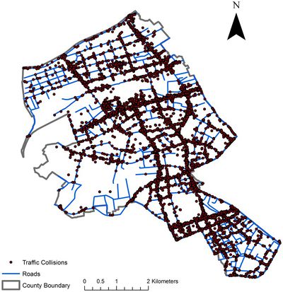
Traffic accident point events were separated from casualty point events before removing duplicates. Unique accident points allow for visualization of intensity and spatial distribution of traffic accidents. Standardization of data, such as, ensuring columns of each CSV files and their data types are the same before reclassifying selected columns, is conducted.
Data Transformation
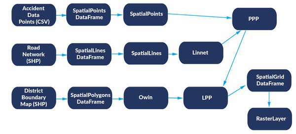
As our geospatial application involves the use of Network Constrained analyses, data has to be transformed to appropriate formats before relevant functions could be used. Specifically, accident traffic points have to be converted to SpatialPoints and then to Point Pattern Processes. Roads would have to be converted to SpatialLines and then to Linnet before they could be combined with Point Patterns Processes to form Linear Point Patterns. In order to constrain the Linear Point Patterns to a target area of interest, it has to be intersected with the Owin of District Boundary Map. The below figure summarises the key data transformation that takes place.
LITERATURE REVIEW
1. Network-constrained spatio-temporal clustering analysis of traffic collisions in Jinghan District of Wuhan, China
(By: Yaxin Fan, Xinyan Zhu, Bing She, Wei Guo, Tao Guo)
Aim of Study: To explore the spatio-temporal clustering patterns of traffic collisions by combining a set of network-constrained methods.
Methodology:
- Weighted network kernel density estimation
- Provides an intuitive way to incorporate attribute information
- Network cross K-function
- Shows that there are varying clustering tendencies between traffic collisions and different types of points of interests (POIs)
- Network differential Local Moran’s I and network local indicators of mobility association
- Provides straightforward and quantitative measures of the hotspot changes
Learning Points:
- Taking into consideration of contributory factors that may affect or correlate with the occurrence of traffic collisions (using network cross K-function to quantify spatial interrelationships between two types of point sets, coupled with Monte Carlo simulation method to test the distribution pattern of point events)
- Incorporated semantic information and temporal dimension of traffic collisions for comprehensive understanding of the spatio-temporal clustering patterns
- Considered POIs that might not directly relate to individual collisions but their spatial distribution might correlate with spatial distribution of collisions collectively
Areas for Improvement:
- Perhaps key implementation issues can be highlighted to allow readers to be aware of the potential drawbacks when implementing the mentioned algorithms, and to make necessary changes according to their context.
2. Visualizing Traffic Accident Hotspots Based on Spatial-Temporal Network Kernel Density Estimation
(By: Benjamin Romano, Zhe Jiang)
Aim of Study: Using Spatial-Temporal Network Kernel Density Estimation To Analyse Traffic Accidents in New York
Methodology:
- Spatio-temporal network kernel density estimation (STNKDE)
- In Network Kernel Density Estimation, edges are split into lixels. STNKDE extends the concept of lixel to include a temporal aspect.
Learning Points:
- Use of spatial-temporal methods helps to avoid over-allocation of resources during non-peak hours
Areas for Improvement:
- Explore the use of combining Getis-Ord GI* statistics to determine if hotspots are statistically significant
- Perhaps apply the spatial-temporal aspects to other relevant methods such as Weighted Kernel Density Estimation
3. Analysis of data on the dataset of road accidents in Paris in 2012 and 2013
http://www.remyzum.com/shiny/Paris_Accidentologie/ (By: Remy Zumbiehl)
Aim of Study: Exploratory data analysis of road accident in Paris
Methodology:
- Basic Mapping using Leaflet Package
Learning Points:
- Using different symbol or marker to present the severity of the road accidents
- Adding filters to drill down the dataset
- Types of vehicles
- Temporal Analysis - date range, the day of the week and time frame
Areas for Improvement:
- Add in geospatial analysis such as Kernel Density Estimation and Network Constrained Analysis
APPROACH
After analysing several literature reviews, it is clearly inappropriate to use the standard point pattern analysis used for two-dimensional space. Our analyses need to take into account the geometry of the network and as such, we have to constrain statistical techniques such as K-Function to the network. We will first delve into uncovering which road segments have a higher intensity of road accidents followed by using various network-constrained techniques to investigate if there are statistically significant clusters.
1. Network Constrained Kernel Density Estimation
Kernel Density Estimation involves estimating the probability density function of a variable, or in other words the density of features in a neighbourhood in geospatial terms. Investigating the average density of points along the network provides a quick insight on which segments of roads has higher intensity of traffic accidents.
There are two main types of intensities when estimating kernel densities in networks:
- Homogeneous intensity function has randomness that is characterised by complete spatial randomness. All points are independent and uniformly distributed in any given set.
- Inhomogeneous intensity function also has independence between disjoint sets but points are unevenly distributed according to their spatially varying intensity functions.
Homogeneous intensity is used as traffic accidents are assumed to occur in spatial randomness. The kernel estimate of intensity has the form:
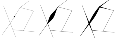
k(v,u) is the smoothing kernel to smooth out a point on the network, as shown below, in a book by Adrian et al (2016). The smoothing of the point is done with a Gaussian kernel and thickness of line proportional to the kernel value. This can be performed using the density.lpp function in R.
2. Second-Order Network Constrained K-Function (Network Constrained Ripley's K-Function)
After gaining insight on the density of traffic accidents, we would take the next step to uncover if the point patterns are dispersed, clustered or randomly distributed. This could be done using Network K-Function.
The Okabe-Yamada network K-Function defines the Network K-Function, by adapting the Ripley’s K Function through replacing the Euclidean distance with the shortest path distance. In this method, given a point v on the network, all locations in the network that can be reached from v by a path of length shorter than a radius r, defined by the user, would be considered. It is defined by the function below, with lambda(L) denoting the total length of the linear network :
While the above Network K-Function constrains points to networks, a second-order stationary point process is required for our analyses. The Okabe-Yamada network K-Function assumes that the network itself is homogeneous, which is not the case as different locations in the network is surrounded by different configurations of line segments. Network K-Functions obtained from different networks are not directly compatible in this case.
The second-order Network K-Function is proposed by Ang et al (2012) , known as the ‘geometrically corrected K-Function’. It is an extension of the Ripley’s K-Function’s benefits of enabling comparison between different point processes with different intensities, observed in different windows, combined with Okabe-Yamada network K-function. The geometrically corrected K-Function is defined by, for all r ≤ R, where u is any location on the network:
The above analysis can be computed in spatstat by the function linearK. It is noted that K-Function assumes homogeneity.
3. Correlation in Multitype Point Patterns Using Network Constrained Cross K-Function
Network Constrained K-Function handles points of the same type while Network Constrained Cross-K Function is used for two different sets of points. Estimation is based on measuring pairwise distances from all points of type i to all points of type j. Thus, for any pair of types i and j, the function calculates the expected number of points of type j lying within a distance r of a typical point of type i, standardised by dividing the intensity of points of type j, for r >= 0. The Cross-K Function is as shown below and it is constrained to a network in our application.
This can be implemented in R through the function linearKcross.
4. Correlation in Multitype Point Patterns Using Network Constrained Cross Pair Correlation
Similar to Network Constrained Cross K-Function, Network Constrained Cross Pair Correlation Function measures pairwise distances from all points of type i to all points of type j. However, this function calculates the expected number of points of type j lying at a distance equal to distance r of a typical point of type i, standardised by dividing the intensity of points of type j, for r >= 0. The cross pair correlation function is as shown below, and it is constrained to a network in our application.
This analysis is computed in spatstat by the function linearpcfcross.
STORYBOARD
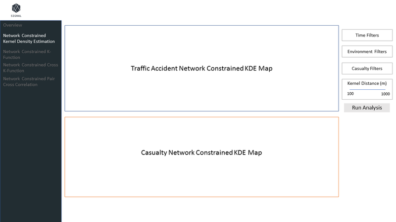
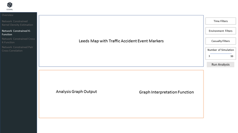
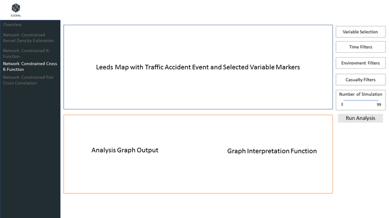
After rounds of refinement, below are the storyboard of our application:
Network Constrained KDE page
Network Constrained KDE page will have 2 maps to show traffic accidents and casualty KDE to allow the user to compare the map. Filters and a kernel distance slider will be at the right-hand side of the application.
Network Constrained K-Function page
Network Constrained K-Function page will have a map at the top and a result box at the bottom which consists of the analysis graph output along with the interpretation function of the graph. Filters and simulation slider will be at the right-hand side of the application.
Network Constrained Cross K-Function and Network Constrained Cross Pair Correlation Function page
Network Constrained Cross K-Function and Network Constrained Cross Pair Correlation Function page will have a map at the top and a result box at the bottom which consists of the analysis graph output along with the interpretation function of the graph. Filters, a variable selection dropdown bar and simulation slider will be at the right-hand side of the application.
TOOLS & TECHNOLOGIES
Tools and technologies
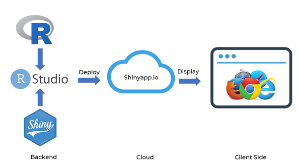
Data Architecture
APPLICATION OVERVIEW
Network Constrained Kernel Density Estimation
Other Network Constrained Analysis
Network Constrained K-Function, Network Constrained Cross K-Function and Network Constrained Cross Pair Correlation Function have the same layout.
| Component | Purpose |
|---|---|
| Leeds Map |
The markers are to indicate the geographical positions of traffic accidents and other variables (Pedestrian Crossing, Motorway Junctions and Schools). The user is able to zoom in and move the map using the map control button to an area that they wish to run the analysis on. |
| Kernel Density Estimation Maps |
The user is able to zoom in and move the map using the map control button to an area that they wish to run the analysis on. When the user move or zoom into the top map, the bottom map will be updated automatically as both maps are sync together. This is to ensure that the analysis on both maps are at the same geographical area so that the user is able to have a fair comparison between both maps. |
| Time Filters |
The user will be able to filter the data by year, month and hours. |
| Environment Filters |
The user will be able to filter the data by:
|
| Casualty Filters |
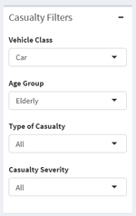
The user will be able to filter the data by:
|
| Kernel Distance Slider |
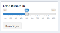
The bandwidth of kernel density plot. The user is able to drag the slider to state the kernel distance in metre which they want to run for the analysis. |
| Simulation Slider |
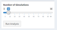
The user is able to drag the slider to state the number of simulations which they want to run for the analysis. |
| Variable Selection |
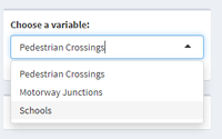
The user is able to choose which variable they want to run the analysis with the traffic accidents. This variable selection is only for Network Constrained Cross K-Function and Network Constrained Cross Pair Correlation Function analysis. |
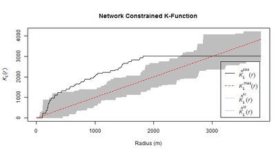
| Network Constrained K-Function |
Output for Network Constrained K-Function Analysis |
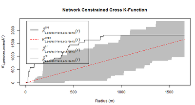
| Network Constrained Cross K-Function |
Output for Network Constrained Cross K-Function Analysis |
| Network Constrained Cross Pair Correlation Function |
Output for Network Constrained Cross Pair Correlation Function Analysis |
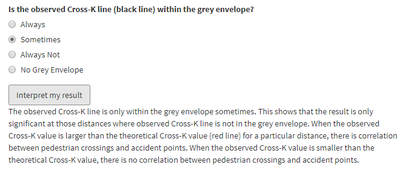
| Graph Interpretation Function |
The user will choose an option according to the graph output and a general interpretation will be shown on the application. The graph interpretation function is to aid the user to interpret the graph output. This graph interpretation function will be placed in all analysis except Network Constrained KDE. |
INSIGHTS
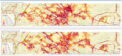
When it comes to traffic accidents, it is instinctive for most people to only focus on the traffic accidents KDE to identify areas with high intensity of accidents and overlook the concentration of casualty points. For instance, if the authorities are looking into reducing the number of elderly casualties, naturally, they will focus on areas with high intensity of traffic accidents. However, that may not be representative of the age group that they are targeting. Thus, the solution provided two different network constrained KDE maps, one focusing on traffic accidents as a whole and the other focusing on the casualties.
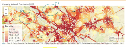
In above figure, although the intensities of the two maps are not strikingly different, there are notable areas that can be focused on. In the first circled area (denoted as (1)), the intensity of traffic accidents are relatively high, however, the intensity of casualties is the opposite. This indicates that if the authorities are focusing on reducing elderly casualties, they should not be focusing all their resources in this area. Instead, they should be focusing in areas with higher intensity of casualty, but were not so apparent when looking at the intensity of traffic accident, as shown in the second circled area (denoted as (2)). In (2), it is shown that there are relatively low traffic accidents happening in at area, however, the intensity of elderly casualties are quite high. This serves to show that the authorities should be focusing on this area, should their primary goal be reducing the number of accidents involving elderly casualties.
After analysing the intensity of traffic accidents, authorities can proceed to investigate if there are signs of traffic accident clusters or correlation patterns between variables such as pedestrian crossings and traffic accident points in a selected road segment. These results are drawn from Network Constrained K-Function, Network Constrained Cross K-Function and Network Constrained Cross Pair Correlation in our application. Subsequent discussions on results is focused on the city centre of Leeds, where Network Constrained Kernel Density Estimation has pointed out as having consistently high intensity of traffic accidents.
Network Constrained K-Function has proved that there is evidence of statistically significant clustering of traffic accidents involving all types of elderly casualties in the north of city centre for most distances along Inner Ring Road and The Headrow Road, as shown in above figure.
Network Constrained Cross K-Function revealed evidence of correlation between pedestrian crossings and elderly for most of the distances along The Headrow Road and Woodhouse Lane, peaking at 800m (seen in below figure). This means that accidents involving elderly tend to occur near pedestrian crossings more often than random. Authorities aiming to investigate traffic accidents involving elderly could look into this road segment, paying special attention to pedestrian crossings.
While Network Constrained Cross Pair Correlation offers an alternative to computing correlation, there are instances where its results contradicts that of Network Constrained Cross K-Function. As shown below, pedestrian crossings and elderly casualties appear to correlate significantly at smaller distances (about 200m and below), while they do not correlate significantly at large distances (about 1200m and above). This differs from our findings with Network Constrained Cross K-Function, which shows that pedestrian crossings and elderly tends to correlate at larger distances.
KEY CHALLENGES
The following are some of the key technical challenges that we may face throughout the course of the project:
| Key Challenges | Mitigation Plan |
|---|---|
| Unfamiliarity with spatial analysis methods related to network constrained |
|
| Unfamiliarity with Rshiny |
|
| Unfamiliarity with Leeds geographical area |
|
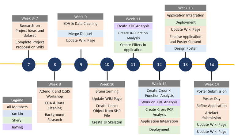
TIMELINE
REFERENCES
- Chua, A. (2018, February 7). Fatal road accidents and fatalities hit all-time low in 2017: Traffic Police. Retrieved from https://www.todayonline.com/singapore/fatal-road-accidents-and-fatalities-hit-all-time-low-2017-traffic-police
- Fan, Y., Zhu, X., She, B., Guo, W. & Guo, T. (2018) Network-constrained spatio-temporal clustering analysis of traffic collisions in Jianghan District of Wuhan, China. PLoS ONE 13(4): e0195093. Retrieved from https://doi.org/10.1371/journal.pone.0195093
- Rui, Y., Yang, Z., Qian T., Khalid, S., Xia N. & Wang J. (2016) Network-constrained and category-based point pattern analysis for Suguo retail stores in Nanjing, China. Retrieved from https://doi.org/10.1080/13658816.2015.1080829
- Turner, A. (2018, November 13). How Big Data is Driving Innovation in the Leeds City Region. Retrieved from https://leeds-list.com/discussion/how-big-data-is-driving-innovation-in-the-leeds-city-region/
- Xie, Z. & Yan, J. (2008). Kernel Density Estimation of traffic accidents in a network space. Computers, Environment and Urban Systems, 32, 396-406. Retrieved from https://doi.org/10.1016/j.compenvurbsys.2008.05.001
- Yamada, I. & Thill, J. (2010). Local Indicators of Network-Constrained Clusters in Spatial Patterns Represented by a Link Attribute. Annals of the Association of American Geographers. 100. 269-285. Retrieved from https://doi.org/10.1080/00045600903550337
- Zumbiehl, R (2018, October 16). Accidentology in Paris. Retrieved from http://www.remyzum.com/shiny/Paris_Accidentologie/
COMMENTS
Feel free to leave us some comments so that we can improve!
| No. | Name | Date | Comments |
|---|---|---|---|
| 1. | Insert your name here | Insert date here | Insert comment here |
| 2. | Insert your name here | Insert date here | Insert comment here |
| 3. | Insert your name here | Insert date here | Insert comment here |


