Difference between revisions of "EzModel Proposal"
| (36 intermediate revisions by 2 users not shown) | |||
| Line 49: | Line 49: | ||
<tr> | <tr> | ||
<td> 2014 Master Plan Planning Subzone (Web) </td> | <td> 2014 Master Plan Planning Subzone (Web) </td> | ||
| − | <td> [https://data.gov.sg/dataset/master-plan-2014-subzone-boundary-web | + | <td> [https://data.gov.sg/dataset/master-plan-2014-subzone-boundary-web Data.gov.sg] </td> |
<td> SHP </td> | <td> SHP </td> | ||
</tr> | </tr> | ||
<tr> | <tr> | ||
<td> HDB Resale Flat Prices Dataset </td> | <td> HDB Resale Flat Prices Dataset </td> | ||
| − | <td> [https://data.gov.sg/dataset/resale-flat-prices | + | <td> [https://data.gov.sg/dataset/resale-flat-prices Data.gov.sg] </td> |
<td> SHP<br/>Data was converted from CSV to Shapefile after geocoding HDB Addresses using | <td> SHP<br/>Data was converted from CSV to Shapefile after geocoding HDB Addresses using | ||
| − | [https://docs.onemap.sg/#search | + | [https://docs.onemap.sg/#search OneMap API] and further processing </td> |
</tr> | </tr> | ||
<tr> | <tr> | ||
<td> Pre-School Locations </td> | <td> Pre-School Locations </td> | ||
| − | <td> [https://data.gov.sg/dataset/pre-schools-location | + | <td> [https://data.gov.sg/dataset/pre-schools-location Data.gov.sg] </td> |
<td> KML <br/> Converted to Shapefile</td> | <td> KML <br/> Converted to Shapefile</td> | ||
</tr> | </tr> | ||
<tr> | <tr> | ||
<td> Primary/Secondary School Locations </td> | <td> Primary/Secondary School Locations </td> | ||
| − | <td> [https://data.gov.sg/dataset/school-directory-and-information | + | <td> [https://data.gov.sg/dataset/school-directory-and-information Data.gov.sg] </td> |
<td> CSV<br/>Data was geocoded using | <td> CSV<br/>Data was geocoded using | ||
| − | [https://docs.onemap.sg/#search | + | [https://docs.onemap.sg/#search OneMap API] </td> |
</tr> | </tr> | ||
<tr> | <tr> | ||
| − | <td> | + | <td> MRT/LRT Station Locations </td> |
| − | <td> [ | + | <td> [https://www.mytransport.sg/content/dam/datamall/datasets/Geospatial/TrainStation.zip LTA Datamall] <br/>(Direct Download) </td> |
| − | <td> | + | <td> SHP </td> |
</tr> | </tr> | ||
<tr> | <tr> | ||
| − | <td> | + | <td> Supermarket Locations </td> |
| − | <td> [ | + | <td> [https://data.gov.sg/dataset/supermarkets Data.gov.sg] </td> |
| − | <td> | + | <td> KML <br/> Converted to Shapefile </td> |
| − | |||
</tr> | </tr> | ||
<tr> | <tr> | ||
| + | <td> Shopping Mall Locations </td> | ||
| + | <td> [https://en.wikipedia.org/wiki/List_of_shopping_malls_in_Singapore Wikipedia] </td> | ||
| + | <td> Text <br/> Data was converted to Shapefile after geocoding using | ||
| + | [https://docs.onemap.sg/#search OneMap API] </td> | ||
| + | </tr> | ||
<tr> | <tr> | ||
| − | <td> | + | <td> Park Locations </td> |
| − | <td> [https:// | + | <td> [https://data.gov.sg/dataset/nparks-parks Data.gov.sg] </td> |
| − | <td> | + | <td> KML <br/> Converted to Shapefile </td> |
| + | </tr> | ||
| + | <tr> | ||
| + | <td> Sports Facilities Locations </td> | ||
| + | <td> [https://data.gov.sg/dataset/sportsg-sport-facilities Data.gov.sg] </td> | ||
| + | <td> KML <br/> Converted to Shapefile </td> | ||
</tr> | </tr> | ||
<tr> | <tr> | ||
| − | </tr></table> | + | <td> Hawker Centre Locations </td> |
| + | <td> | ||
| + | Public Food Centres: <br> | ||
| + | 1. [https://data.gov.sg/dataset/hawker-centres Data.gov.sg]<br><br> | ||
| + | Private Food Centres: <br> | ||
| + | 2. [http://www.kopitiam.biz/search-results/?keywords&zone=allzone&FC=yes&search=Search Kopitam]<br> | ||
| + | 3. [https://www.koufu.com.sg/our-brands/food-halls/koufu/ Koufu]<br> | ||
| + | 4. [https://www.foodjunction.com/outlets/ Food Junction]<br> | ||
| + | 5. [https://foodrepublic.com.sg/food-republic-outlets/ Food Republic] | ||
| + | </td> | ||
| + | <td> | ||
| + | 1: KML - Converted to Shapefile <br> | ||
| + | 2 - 5: Text - Data scraped from sites and geocoded using [https://docs.onemap.sg/#search OneMap API] | ||
| + | </td> | ||
| + | </tr> | ||
| + | </table> | ||
As the purpose of the application is to allow users to input their own data into the model, the above data, with the exception of the Master Plan Planning Subzone data and HDB Resale data, will all be loaded onto the server for users without their own data to try out the application. | As the purpose of the application is to allow users to input their own data into the model, the above data, with the exception of the Master Plan Planning Subzone data and HDB Resale data, will all be loaded onto the server for users without their own data to try out the application. | ||
| − | + | <p> | |
| + | Other data preparation steps that had to be performed on the HDB Resale Data included generating a new variable, Storey Median, from the Storey Range column that was provided. For example, a Storey Range of "04 to 06" was converted to a Storey Median value of 5. | ||
| + | </p> | ||
==<div style="background: #FFFFFF; padding-top: 20px; padding-bottom: 20px; line-height: 0.1em; text-indent: 3px; font-size:24px; font-family:Open Sans, Arial, sans-serif; border-bottom:solid #60c0a8;">Literature Review</div>== | ==<div style="background: #FFFFFF; padding-top: 20px; padding-bottom: 20px; line-height: 0.1em; text-indent: 3px; font-size:24px; font-family:Open Sans, Arial, sans-serif; border-bottom:solid #60c0a8;">Literature Review</div>== | ||
=== The Amaize-ing Corn === | === The Amaize-ing Corn === | ||
| − | [https://wiki.smu.edu.sg/18191isss608g1/ISSS608_Group07_Proposal | + | [https://wiki.smu.edu.sg/18191isss608g1/ISSS608_Group07_Proposal View the Project Here]<br><br> |
'''Aim of study'''<br> | '''Aim of study'''<br> | ||
Explore the meteorology and geographical factors that makes a corn in USA, the a-maize-ing crop that we know today | Explore the meteorology and geographical factors that makes a corn in USA, the a-maize-ing crop that we know today | ||
| − | [[File:1024px-DashboardView Group7.png| | + | [[File:1024px-DashboardView Group7.png|200px|frame|center]] |
<br> | <br> | ||
| Line 114: | Line 140: | ||
<br> | <br> | ||
=== CrimeModeler === | === CrimeModeler === | ||
| − | [https://wiki.smu.edu.sg/1718t1isss608g1/ | + | [https://wiki.smu.edu.sg/1718t1isss608g1/Group11_Report View the Project Here] <br><br> |
'''Aim of study'''<br> | '''Aim of study'''<br> | ||
| Line 171: | Line 197: | ||
Rather than merely plotting the results of the user-customised model in a point map form, coloured by R-squared values of the individual regression models around each point, we wish to convey more information. This information is in the form of highlighting regions in which a certain coefficient estimate is greater in scale than other regions. For example, resale prices around a certain HDB town or subzone could be more affected by the number of primary schools around the flats, compared to other regions. | Rather than merely plotting the results of the user-customised model in a point map form, coloured by R-squared values of the individual regression models around each point, we wish to convey more information. This information is in the form of highlighting regions in which a certain coefficient estimate is greater in scale than other regions. For example, resale prices around a certain HDB town or subzone could be more affected by the number of primary schools around the flats, compared to other regions. | ||
<br><br> | <br><br> | ||
| − | Hence, to convey such information to users, we will adopt the use of an isoline map to show regions of high/low coefficients of a user-specified variable. Through interpolating the individual points’ coefficient estimates of the selected variable via | + | Hence, to convey such information to users, we will adopt the use of an isoline map to show regions of high/low coefficients of a user-specified variable. Through interpolating the individual points’ coefficient estimates of the selected variable via an inverse distance weighting method, a surface containing the interpolated data across the entire map area can be layered onto the output display. |
| + | <br> | ||
| + | |||
| + | ==<div style="background: #FFFFFF; padding-top: 20px; padding-bottom: 20px; line-height: 0.1em; text-indent: 3px; font-size:24px; font-family:Open Sans, Arial, sans-serif; border-bottom:solid #60c0a8;">Storyboard</div>== | ||
| + | Below are the storyboards that will be used to guide our design of the application:<br> | ||
| + | {| class="wikitable" | ||
| + | |- | ||
| + | | [[File:EzModel_UploadData.png|500px|User uploads data]]<br> | ||
| + | Tab 1: User uploads data | ||
| + | || [[File:EzModel DefineVars.png|500px|User defines variables]]<br> | ||
| + | Tab 2: User defines variables | ||
| + | |- | ||
| + | | [[File:EzModel ViewData.png|500px|User views data as defined earlier]]<br> | ||
| + | Tab 3: User views data as defined earlier | ||
| + | || [[File:EzModel TransVars.png|500px|User is able to transform data to make it more suitable for regression]]<br> | ||
| + | Tab 4: User is able to transform data to make it more suitable for regression | ||
| + | |- | ||
| + | | [[File:EzModel SelectVars.png|500px|User defines which variables to go into the global/fixed sections in the mixed GWR model]]<br> | ||
| + | Tab 5: User defines variables as global or local | ||
| + | || [[File:EzModel RunGWR.png|500px|User runs calibrated model and views results]] | ||
| + | Tab 6: User runs calibrated model and views results | ||
| + | |} | ||
| + | <br> | ||
| + | ==<div style="background: #FFFFFF; padding-top: 20px; padding-bottom: 20px; line-height: 0.1em; text-indent: 3px; font-size:24px; font-family:Open Sans, Arial, sans-serif; border-bottom:solid #60c0a8;">Application Architecture and Overview</div>== | ||
| + | {| | ||
| + | |[[File:Apparchitecture.jpg|400px|right|thumb|EzModel Application Architecture Diagram]] || <p> | ||
| + | The team developed the application using the R Shiny web application framework that is based on the R programming language. This gave us access to many in-built functions as well as external packages that were built in R, allowing us to perform the many analyses such like the GWR and MGWR required. Packages built for R Shiny also allowed us easy construction of the applications user interface and back-end processing of inputs. | ||
| + | </p> | ||
| + | <p> | ||
| + | The R Shiny application runs on a Shiny server, currently hosted by Shinyapps.io. Data mentioned in Section 3.1 are stored on the server and loaded by the application each time a user accesses the app. The mapping features of the app also makes calls to OpenStreetMap to generate the interactive maps that are displayed to the user. | ||
| + | </p> | ||
| + | |} | ||
| + | {| class="wikitable" | ||
| + | |- | ||
| + | ! App View!! Description | ||
| + | |- | ||
| + | | <strong>Uploading Data</strong> [[File:UploadDataTab.png|500px|left]]|| This tab allows users to upload their own CSV/Shapefiles containing the location data of features of interest that they wish to use to calculate variables that could influence resale prices. Upon upload, a data table shows the users the data that was uploaded, as well as the locations of the data points on an interactive map so that users can verify that the data they uploaded was correctly processed. | ||
| + | |- | ||
| + | | <strong>Choosing Datasets</strong>[[File:ChooseDatasets.png|500px|left]]|| The same "Upload Data" tab also allows users to select our preloaded datasets, as well as their own user-uploaded datasets to be used to for calculations in the later steps. | ||
| + | |- | ||
| + | | <strong>Defining Variables and Filtering/Sampling Data</strong>[[File:DefiningVars.png|500px|left]]|| <p>This tab allows users to filter/sample data from specified time periods. The use of sampling is due to the fact that the GWR and MGWR analyses require long processing times if there were to be thousands of records.</p><p>The slider inputs shown are for users to define the radius in which to calculate the number of features around each observation of a HDB resale transaction, i.e. calculate number of primary schools within 500m radius of each HDB flat recorded in the resale data.</p> | ||
| + | |- | ||
| + | | <strong>Viewing HDB Resale Data and Variable Values</strong> | ||
| + | [[File:ViewDataTab.png|500px|left]] | ||
| + | || Here, users are presented the overall data table of HDB Resale Data, along with appended columns of calculated variables such as the Distance to Nearest <Feature> as well as the Number of <Features> within X radius (where X was defined in the previous tab, as described above). | ||
| + | |- | ||
| + | |<strong>Transforming Variables</strong> | ||
| + | [[File:TransformVars.png|500px|left]]<br> | ||
| + | <em>Transformation Process</em> | ||
| + | [[File:TransformHisto.png|240px|left]] | ||
| + | [[File:LogResalePriceHisto.png|240px|right]] | ||
| + | || The "Transform Variables" tab allows users to view histogram plots and determine if the distribution of the variable's values are skewed or not. If skewed, the user can then define ways to transform the values (e.g. Log, Square Root etc.), such as to make the distribution less skewed/more normal. | ||
| + | |- | ||
| + | | <strong>Selecting Variables for GWR</strong> | ||
| + | [[File:SelectVars.png|500px|left]]<br> | ||
| + | <em>Correlation Plot</em> | ||
| + | [[File:CorrPlot.png|300px|left]] | ||
| + | || <p>Users can now select which variables in the earlier data table, will go into the regression model. Any variable (local/global) will be included in the basic GWR analysis. Whereas in the Mixed GWR analysis, only the Local variables are given spatial variation in their coefficient estimates.</p> | ||
| + | <p>A correlation plot button also allows users to generate a correlation plot between all the variables. This allows users to detect if there are any highly correlated variables already in the model, which may affect the coefficient estimates should there be highly correlated variables inside the model.</p> | ||
| + | |- | ||
| + | | <strong>GWR Results</strong> | ||
| + | [[File:RunGWR.png|500px|left]] | ||
| + | || <p>The final tab allows users to customise their bandwidth as well as kernel functions, before finally running the GWR and mixed GWR (if applicable) analyses. Upon completion of the regression analyses, the results are displayed in isoline maps to show the variation of coefficient estimates/intercept values as well as predicted values across Singapore. The right isoline map also displays local R-square in an isoline map to show how much of the current model is able to explain variation in resale prices at different parts of Singapore. It is layered with p-value map to show areas where the model's estimates are significant/non-significant.</p> | ||
| + | <p>There are multiple tabs inside this view that also allows users to access the Mixed GWR results, which displays similar information, as well as download the output data that was generated from the analyses. Diagnostic information of the different regression models are also available to users to view to compare which models are a better fit.</p> | ||
| + | |} | ||
| + | <br> | ||
| + | |||
| + | ==<div style="background: #FFFFFF; padding-top: 20px; padding-bottom: 20px; line-height: 0.1em; text-indent: 3px; font-size:24px; font-family:Open Sans, Arial, sans-serif; border-bottom:solid #60c0a8;">Results</div>== | ||
| + | The team used some of the preloaded datasets to conduct analysis. The variables that are used are: | ||
| + | {| class="wikitable" | ||
| + | |- | ||
| + | ! Global Variables !! Local Variables | ||
| + | |- | ||
| + | | Floor_Area_SQM || Preschools | ||
| + | |- | ||
| + | | Storey_Median || MRT_LRT_Stations | ||
| + | |- | ||
| + | | Remaining_Lease || Primary_School | ||
| + | |- | ||
| + | | Shopping_Malls || | ||
| + | |- | ||
| + | | CBD_RafflesPlace || | ||
| + | |- | ||
| + | |} | ||
| + | The radius for primary schools in the vicinity of resale HDB units was increased to 1000m. Transformation was also performed on selected sets of the variables. | ||
| + | <table class="wikitable"> | ||
| + | <tr><th colspan=2>Transformation</th></tr> | ||
| + | <tr><th>Log</th><th>Square Root</th></tr> | ||
| + | <tr><td>Resale_Price</td><td>Dist2Nearest_MRT_LRT_Stations</td></tr> | ||
| + | <tr><td>Storey_Median</td><td>Dist2Nearest_Shopping_Malls</td></tr> | ||
| + | <tr><td>Remaining_Lease</td><td>Within1000Radius_Primary_Schools</td></tr> | ||
| + | <tr><th colspan=2>No Transformation</th></tr> | ||
| + | <tr><td>Within500Radius_Preschools</td><td>Floor_Area_SQM</td></tr> | ||
| + | </table> | ||
| + | The kernel function used was set as the default Gaussian and auto bandwidth was used. The results obtained was as follow: | ||
| + | <table class="wikitable"> | ||
| + | <tr> | ||
| + | <th>MLR</th> | ||
| + | <th>GWR</th> | ||
| + | <th>MGWR</th> | ||
| + | </tr> | ||
| + | <tr> | ||
| + | <td>R-square: 67.13% | ||
| + | Adj R-square: 66.6% | ||
| + | <br> | ||
| + | AICc: -702.764 | ||
| + | <br> | ||
| + | All variables significant at 90% CL | ||
| + | </td> | ||
| + | <td>R-square: 88.67% | ||
| + | Adj R-square: 84.32% | ||
| + | <br> | ||
| + | AICc: -964.8 | ||
| + | </td> | ||
| + | <td> | ||
| + | AICc: -982.9 | ||
| + | </td> | ||
| + | </tr> | ||
| + | </table> | ||
| + | <table> | ||
| + | <tr> | ||
| + | <td> | ||
| + | [[File:SqrtDistCoeffResults.png|400px|left|Plot of Local Coefficient of sqrt_distance2nearest_shopping_malls (GWR)|thumb]] | ||
| + | </td> | ||
| + | <td> | ||
| + | <p>The GWR reveals that in areas nearer to CBD and the East, the housing prices are actually more sensitive to the distance to nearest shopping mall (Fig. 20). There is a greater decrease in price as the distance to the nearest shopping mall increase from a HDB resale flat. This possible suggests that buyers looking for flats within these regions view convenient access to shopping as higher priority when making decisions. Given the density of shopping options within these regions, especially in the central areas, it is no surprise that buyers looking at these locations are likely to be more interested in the shopping options aspect when buying a flat, and hence willing to pay greater premiums for for closer and more convenient access to suit their preferences. | ||
| + | </p><p> | ||
| + | It can be further noted that there are some regions that present a positive correlation between resale prices and distance to nearest shopping mall. Possible reasons for this include buyers looking at these areas show less interest towards having convenient shopping options. Another likely possibility that buyers do not see distance to shopping malls as a disadvantage could be due to affluence whereby they are more likely to use ways of transport such as driving, to get to shopping malls. In such a case, being close to a shopping mall is not such a great incentive as compared to individuals who have a preference for walkable distances to their shopping options. | ||
| + | </p> | ||
| + | </td> | ||
| + | </tr> | ||
| + | </table> | ||
| + | |||
| + | <table> | ||
| + | <tr> | ||
| + | <td> | ||
| + | [[File:1kDist2MRT.png|400px|thumb|left|GWR Plot of Local Coefficient of Sqrt Distance to Nearest MRT/LRT Variable]] | ||
| + | </td> | ||
| + | <td><p> | ||
| + | Looking at a different variable, Distance to Nearest MRT/LRT Station, a different distribution of coefficient estimates can be observed. Especially noticeable is the south-west region, where resale flat buyers are more sensitive to a flat’s distance to the nearest MRT station. This presents different possible insights, depending on perspective. Firstly, this could be an indication of a high demand for access to the MRT stations along that area, which stretches from stations such as Clementi, up till Tanjong Pagar/Raffles Place. Given the heavy peak-hour demands of the East-West line and its direct access to the bustling city centre where many offices are located at, it is not surprising that having access to the stops along this MRT line will bring about greater convenience to buyers of houses near these stations. Another perspective could be that access to these MRT stations via vehicular transport options may not be convenient. For example, overcrowded buses to/from MRT stations during peak hours could be a factor that incentivise commuters to walk instead. As such, buyers are more willing to pay greater premiums for nearer distances to MRT stations in these areas. | ||
| + | </p><p> | ||
| + | However, in Fig. 21, in the eastern regions around Bedok, it can also be observed that there is positive correlation between resale price and distance to nearest MRT station. A reason for this could be that there are few MRT transport options within that region, and buyers who are looking for properties in this region do not see accessibility to MRT transport as an important factor. Instead, transport via buses could suffice. The points located near the East Coast Park region, near to the coast, could be evidence that connectivity to the MRT network is not a priority for the buyers of those resale flats.</p> | ||
| + | </td> | ||
| + | </tr> | ||
| + | </table> | ||
| + | <p> | ||
| + | Comparing the AICc values of the models, it is shown that GWR is far more superior in performance as compared to the MLR and MGWR was also slightly better than the GWR due to the rendering of variables that does not have too much spatial variations. | ||
| + | </p> | ||
| + | <table> | ||
| + | <tr> | ||
| + | <td>[[File:SqrtDistMRTResults.png|400px|thumb|left|MGWR Model on 3-Room Resale HDB]]</td> | ||
| + | <td> | ||
| + | <p>Using the same attributes for the MGWR model on 3 room resale HDB and 5-room resale HDB data yields interesting results. The 5-room HDB resale flats observes a smaller range for the coefficient estimates as compared to the 3-room HDB resale flats. One possible explanation is that 5-room HDB flats occupants and buyers are more wealthy in general and it might be possible that a larger proportion of them have their own family vehicles, making them not be too affect if the nearest MRT/LRT stations are more further away as compared to 3-room HDB flat buyers and occupants.</p></td> | ||
| + | <td>[[File:SqrtDistMRT5roomResults.png|350px|thumb|right|MGWR Model on 5-Room Resale HDB]]</td> | ||
| + | </tr> | ||
| + | </table> | ||
<br> | <br> | ||
==<div style="background: #FFFFFF; padding-top: 20px; padding-bottom: 20px; line-height: 0.1em; text-indent: 3px; font-size:24px; font-family:Open Sans, Arial, sans-serif; border-bottom:solid #60c0a8;">Project Timeline</div>== | ==<div style="background: #FFFFFF; padding-top: 20px; padding-bottom: 20px; line-height: 0.1em; text-indent: 3px; font-size:24px; font-family:Open Sans, Arial, sans-serif; border-bottom:solid #60c0a8;">Project Timeline</div>== | ||
| + | <br> | ||
| + | [[File:Gantt chart.png|1150px|center]] | ||
<br> | <br> | ||
| Line 211: | Line 394: | ||
|- | |- | ||
| gstats || Advanced Geostatistical Techniques: Kriging and Point-Map Overlays | | gstats || Advanced Geostatistical Techniques: Kriging and Point-Map Overlays | ||
| + | |- | ||
| + | |shiny, shinydashboard, shinyWidgets, shinyjs<br>shinycssloaders, shinythemes, shinyBS || R Shiny widgets and UI customisation | ||
| + | |- | ||
|} | |} | ||
<br> | <br> | ||
Latest revision as of 23:02, 14 April 2019

Contents
Project Motivation
In recent decades, modeling housing prices has become a hot topic among economists, planners, and policymakers due to the significant role of properties in household wealth and national economy. In Singapore, public housing accommodates more than 80% of its citizen and citizens either choose to buy a new Housing Development Board (HDB) flat or purchase a HDB resale flat, second-hand flats with less than 99 years left on the lease. Our project will focus on modelling the HDB resale flat prices which are shaped by market forces.
In many existing hedonic housing prices models, linear regression is used to identify the significance of different variables (number of rooms, number of years left on the lease and distance from the nearest amenities etc.) on the house prices. However, these models fail to take into account the spatial variation in the nearby surroundings of these different resale units such as the proximity to shopping malls, number of MRT stations and healthcare facilities in the vicinity.
Geographically weighted regression (GWR) is a spatial analysis technique that overcomes this limitation by taking into account spatial autocorrelations among the observations in surrounding locations by allowing for spatial nonstationarity in the linear regression coefficients for each observation location. In this project, we will build a modeling tool that allows users to explore the impact of these spatial variations on HDB resale prices through a GWR model. To factor in the combination of both local and global variables, we also includes the option of using a mixed (semiparametric) GWR model.
Also, to provide greater flexibility for users to choose the certain desired spatial attributes that they would like to analyse, instead of fixing the datasets to be used for the model, we will allow users to upload datasets (i.e. school locations, hospital locations) and the tool will immediately compute new spatial variables for users to include in the model for analysis. This tool thus seeks to help users to accurately model the impact of spatial variables on the price of the HDB resale units.
Data Sources
| Data | Source | Data Type/Method |
|---|---|---|
| 2014 Master Plan Planning Subzone (Web) | Data.gov.sg | SHP |
| HDB Resale Flat Prices Dataset | Data.gov.sg | SHP Data was converted from CSV to Shapefile after geocoding HDB Addresses using OneMap API and further processing |
| Pre-School Locations | Data.gov.sg | KML Converted to Shapefile |
| Primary/Secondary School Locations | Data.gov.sg | CSV Data was geocoded using OneMap API |
| MRT/LRT Station Locations | LTA Datamall (Direct Download) |
SHP |
| Supermarket Locations | Data.gov.sg | KML Converted to Shapefile |
| Shopping Mall Locations | Wikipedia | Text Data was converted to Shapefile after geocoding using OneMap API |
| Park Locations | Data.gov.sg | KML Converted to Shapefile |
| Sports Facilities Locations | Data.gov.sg | KML Converted to Shapefile |
| Hawker Centre Locations |
Public Food Centres: |
1: KML - Converted to Shapefile |
As the purpose of the application is to allow users to input their own data into the model, the above data, with the exception of the Master Plan Planning Subzone data and HDB Resale data, will all be loaded onto the server for users without their own data to try out the application.
Other data preparation steps that had to be performed on the HDB Resale Data included generating a new variable, Storey Median, from the Storey Range column that was provided. For example, a Storey Range of "04 to 06" was converted to a Storey Median value of 5.
Literature Review
The Amaize-ing Corn
View the Project Here
Aim of study
Explore the meteorology and geographical factors that makes a corn in USA, the a-maize-ing crop that we know today

Methodology
- Geographically weighted regression to analyse the natural factors that affect corns’ yield
- Inverse Distance Weighted technique to visualise and analyse the natural factors on an isoline map
Learning Points
- Spatial Analysis Techniques
- Learn how to enable users to select and drop variables for geographical weighted modeling on the RShiny Application
- Learn to use the gstat library to plot an isoline map for better analysis of the spatial variables
Area for Improvement
- Possible use of mixed geographically weighted regression model to account for global variables instead of assuming all are local variables in a typical GWR model
CrimeModeler
Aim of study
Examine the relationship of crime and socio-economic characteristics for each district and how crime differs across different districts in England and Wales.
Methodology
- Linear regression (Gaussian error distribution) for feature selection
- Geographically weighted regression (GWR) after obtaining the significant variables from the generalised linear regression. A distance decay function a and the corresponding bandwidth can be specified by the user
Learning Points
- Although the app consists of the a large variety of visualizations and inputs for users to specify, the application still loaded quickly is thus is very interactive with the help of AngularJS
- Ridge penalty is put in during generalised linear regression when no variables are entered.
Area for Improvement
- Unable to specify which variables should be specified as global and which to local, which will fit then model better
Approach
After conducting the literature review, our team is clearer on the approach that our application will have in allowing users to define their overall model.
Collinearity
As users will be working with multiple independent variables, it is undesirable for the model to include independent variables that are high in collinearity with respect to each other as this will result in multicollinearity. Hence, after selecting the variables that the user wants to include in the model, a plot of the correlation matrix between each variable with each other will be available for the user to filter out variables that present high correlation with another variable.
Global Regression
A global regression model using the selected independent variables will be run, with the output of the coefficients estimates as well the resulting t-statistic and p-value used to determine if the independent variable should remain in the model. This would be done based on the criteria set by the user on the confidence level required. Thus, previously selected variables that turn out to be insignificant to the overall model will be excluded to help users derive a more accurate model.
Geographically Weighted Regression
The advantage of using a GWR, as highlighted previously (link to Project Motivation), takes into account spatial nonstationarity in terms of the coefficients of each variable for each observation in the resulting regression model. This results in an equation as such:
Where the intercepts and the coefficients are varied according to the location of the observation and the surrounding observations in the spatial context.
Thus, there are a few parameters that have to be calibrated before running the GWR. Firstly, as different observations will be assigned different weights depending on the location with respect to each point, a weighting kernel function has to be decided upon to determine the allocation of weights to each observation according to distance. This is in contrast with the global function, which gives equal weightage to all observations.
Such kernel functions include:
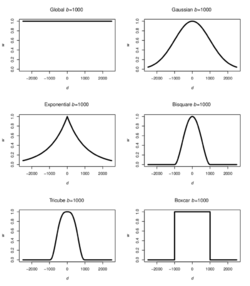
- Gaussian
- Exponential
- Box-car
- Bi-square
- Tri-cube.
The functions can be categorised into two main types: Continuous and Discontinuous. Continuous functions include the Gaussian and Exponential kernels, where weightage decreases gradually as distance increases. Even beyond the determined bandwidth, observations are still assigned a weightage, although the weightage is very small. Whereas discontinuous functions include the Box-car, Bi-square and Tri-cube kernels, whereby observations’ weightages are reduced to zero once distance between observation and the center-point exceeds the specified bandwidth.
Secondly, another parameter that has to be calibrated for the GWR model would be the weighting scheme. In essence, there are two main weighting schemes: Fixed and Adaptive. This is largely tied in with the third parameter to be customised: bandwidth. In a fixed weighting scheme, the same bandwidth is applied to all observations when applying the weighting kernel function. This, however, might cause issues whereby there are lesser observations taken into account in areas where data points are sparse, and more points included in areas where observations are dense. This is where an adaptive weighting scheme applies, in which bandwidth is adjusted according to the context of each observation, for example, to a pre-determined k nearest neighbours. Thus where data points are sparse, bandwidth increases, and where data points are dense, bandwidth is reduced.
Lastly, the method to determining bandwidth also has to be calibrated for the model. Aside from the user entering a pre-defined bandwidth, there are two other possible methods. Firstly, the Least Cross-Validation (CV) score method helps determine a bandwidth based on minimizing squared errors. The other method would be using the Least Akaike Information Criterion (AIC) method that takes into account different degrees of freedom for varying models from the different observations.
Due to the fact that the use of different kernel functions, weighting schemes, as well as bandwidth determination methods will affect the overall GWR model output, we want to give users the ability to calibrate their model based on these parameters based on what they wish to explore, or based on what they deem is most appropriate for the variables selected.
Mixed (Semiparametric) GWR
The mixed GWR model, as suggested by its name, allows for a mix of both analysis variables that will be regressed according to the geographic weights of the observations around it, as well as variables in which coefficients estimates derived from a global regression will be kept constant throughout all observations and resulting models. For example, the coefficient for which the floor range of a flat affects its resale price might be deemed to be/approximately constant throughout observations. Hence, this Floor Range variable could be selected to be a variable in which its coefficient estimate would be globally applied to all the resulting mixed GWR models.
Users can experiment in creating an optimal model by selecting independent variables in which they want the coefficient estimates to be kept global, while leaving the other variables to be run against the GW regression.
Isoline Map

Rather than merely plotting the results of the user-customised model in a point map form, coloured by R-squared values of the individual regression models around each point, we wish to convey more information. This information is in the form of highlighting regions in which a certain coefficient estimate is greater in scale than other regions. For example, resale prices around a certain HDB town or subzone could be more affected by the number of primary schools around the flats, compared to other regions.
Hence, to convey such information to users, we will adopt the use of an isoline map to show regions of high/low coefficients of a user-specified variable. Through interpolating the individual points’ coefficient estimates of the selected variable via an inverse distance weighting method, a surface containing the interpolated data across the entire map area can be layered onto the output display.
Storyboard
Below are the storyboards that will be used to guide our design of the application:
 Tab 1: User uploads data |
 Tab 2: User defines variables |
 Tab 3: User views data as defined earlier |
 Tab 4: User is able to transform data to make it more suitable for regression |
 Tab 5: User defines variables as global or local |

Tab 6: User runs calibrated model and views results |
Application Architecture and Overview
The team developed the application using the R Shiny web application framework that is based on the R programming language. This gave us access to many in-built functions as well as external packages that were built in R, allowing us to perform the many analyses such like the GWR and MGWR required. Packages built for R Shiny also allowed us easy construction of the applications user interface and back-end processing of inputs. The R Shiny application runs on a Shiny server, currently hosted by Shinyapps.io. Data mentioned in Section 3.1 are stored on the server and loaded by the application each time a user accesses the app. The mapping features of the app also makes calls to OpenStreetMap to generate the interactive maps that are displayed to the user. |

| App View | Description |
|---|---|
Uploading Data  |
This tab allows users to upload their own CSV/Shapefiles containing the location data of features of interest that they wish to use to calculate variables that could influence resale prices. Upon upload, a data table shows the users the data that was uploaded, as well as the locations of the data points on an interactive map so that users can verify that the data they uploaded was correctly processed. |
Choosing Datasets |
The same "Upload Data" tab also allows users to select our preloaded datasets, as well as their own user-uploaded datasets to be used to for calculations in the later steps. |
Defining Variables and Filtering/Sampling Data |
This tab allows users to filter/sample data from specified time periods. The use of sampling is due to the fact that the GWR and MGWR analyses require long processing times if there were to be thousands of records. The slider inputs shown are for users to define the radius in which to calculate the number of features around each observation of a HDB resale transaction, i.e. calculate number of primary schools within 500m radius of each HDB flat recorded in the resale data. |
Viewing HDB Resale Data and Variable Values
 |
Here, users are presented the overall data table of HDB Resale Data, along with appended columns of calculated variables such as the Distance to Nearest <Feature> as well as the Number of <Features> within X radius (where X was defined in the previous tab, as described above). |
Transforming Variables
 Transformation Process   |
The "Transform Variables" tab allows users to view histogram plots and determine if the distribution of the variable's values are skewed or not. If skewed, the user can then define ways to transform the values (e.g. Log, Square Root etc.), such as to make the distribution less skewed/more normal. |
Selecting Variables for GWR
 Correlation Plot  |
Users can now select which variables in the earlier data table, will go into the regression model. Any variable (local/global) will be included in the basic GWR analysis. Whereas in the Mixed GWR analysis, only the Local variables are given spatial variation in their coefficient estimates. A correlation plot button also allows users to generate a correlation plot between all the variables. This allows users to detect if there are any highly correlated variables already in the model, which may affect the coefficient estimates should there be highly correlated variables inside the model. |
GWR Results
 |
The final tab allows users to customise their bandwidth as well as kernel functions, before finally running the GWR and mixed GWR (if applicable) analyses. Upon completion of the regression analyses, the results are displayed in isoline maps to show the variation of coefficient estimates/intercept values as well as predicted values across Singapore. The right isoline map also displays local R-square in an isoline map to show how much of the current model is able to explain variation in resale prices at different parts of Singapore. It is layered with p-value map to show areas where the model's estimates are significant/non-significant. There are multiple tabs inside this view that also allows users to access the Mixed GWR results, which displays similar information, as well as download the output data that was generated from the analyses. Diagnostic information of the different regression models are also available to users to view to compare which models are a better fit. |
Results
The team used some of the preloaded datasets to conduct analysis. The variables that are used are:
| Global Variables | Local Variables |
|---|---|
| Floor_Area_SQM | Preschools |
| Storey_Median | MRT_LRT_Stations |
| Remaining_Lease | Primary_School |
| Shopping_Malls | |
| CBD_RafflesPlace |
The radius for primary schools in the vicinity of resale HDB units was increased to 1000m. Transformation was also performed on selected sets of the variables.
| Transformation | |
|---|---|
| Log | Square Root |
| Resale_Price | Dist2Nearest_MRT_LRT_Stations |
| Storey_Median | Dist2Nearest_Shopping_Malls |
| Remaining_Lease | Within1000Radius_Primary_Schools |
| No Transformation | |
| Within500Radius_Preschools | Floor_Area_SQM |
The kernel function used was set as the default Gaussian and auto bandwidth was used. The results obtained was as follow:
| MLR | GWR | MGWR |
|---|---|---|
| R-square: 67.13%
Adj R-square: 66.6%
|
R-square: 88.67%
Adj R-square: 84.32%
|
AICc: -982.9 |
|
The GWR reveals that in areas nearer to CBD and the East, the housing prices are actually more sensitive to the distance to nearest shopping mall (Fig. 20). There is a greater decrease in price as the distance to the nearest shopping mall increase from a HDB resale flat. This possible suggests that buyers looking for flats within these regions view convenient access to shopping as higher priority when making decisions. Given the density of shopping options within these regions, especially in the central areas, it is no surprise that buyers looking at these locations are likely to be more interested in the shopping options aspect when buying a flat, and hence willing to pay greater premiums for for closer and more convenient access to suit their preferences.
It can be further noted that there are some regions that present a positive correlation between resale prices and distance to nearest shopping mall. Possible reasons for this include buyers looking at these areas show less interest towards having convenient shopping options. Another likely possibility that buyers do not see distance to shopping malls as a disadvantage could be due to affluence whereby they are more likely to use ways of transport such as driving, to get to shopping malls. In such a case, being close to a shopping mall is not such a great incentive as compared to individuals who have a preference for walkable distances to their shopping options. |

Looking at a different variable, Distance to Nearest MRT/LRT Station, a different distribution of coefficient estimates can be observed. Especially noticeable is the south-west region, where resale flat buyers are more sensitive to a flat’s distance to the nearest MRT station. This presents different possible insights, depending on perspective. Firstly, this could be an indication of a high demand for access to the MRT stations along that area, which stretches from stations such as Clementi, up till Tanjong Pagar/Raffles Place. Given the heavy peak-hour demands of the East-West line and its direct access to the bustling city centre where many offices are located at, it is not surprising that having access to the stops along this MRT line will bring about greater convenience to buyers of houses near these stations. Another perspective could be that access to these MRT stations via vehicular transport options may not be convenient. For example, overcrowded buses to/from MRT stations during peak hours could be a factor that incentivise commuters to walk instead. As such, buyers are more willing to pay greater premiums for nearer distances to MRT stations in these areas. However, in Fig. 21, in the eastern regions around Bedok, it can also be observed that there is positive correlation between resale price and distance to nearest MRT station. A reason for this could be that there are few MRT transport options within that region, and buyers who are looking for properties in this region do not see accessibility to MRT transport as an important factor. Instead, transport via buses could suffice. The points located near the East Coast Park region, near to the coast, could be evidence that connectivity to the MRT network is not a priority for the buyers of those resale flats. |

Comparing the AICc values of the models, it is shown that GWR is far more superior in performance as compared to the MLR and MGWR was also slightly better than the GWR due to the rendering of variables that does not have too much spatial variations.
|
Using the same attributes for the MGWR model on 3 room resale HDB and 5-room resale HDB data yields interesting results. The 5-room HDB resale flats observes a smaller range for the coefficient estimates as compared to the 3-room HDB resale flats. One possible explanation is that 5-room HDB flats occupants and buyers are more wealthy in general and it might be possible that a larger proportion of them have their own family vehicles, making them not be too affect if the nearest MRT/LRT stations are more further away as compared to 3-room HDB flat buyers and occupants. |


Project Timeline

Challenges
| Key Challenges | Mitigation |
|---|---|
| Unfamiliar with R |
|
| Unfamiliar with the various analysis techniques using packages |
|
| Data obtained and uploaded by users are not in the right format |
|
Tools & Technology
| R Packages | Function |
|---|---|
| sp, sf, rgdal, tidyverse | Data Cleaning and Data Wrangling |
| ggplot2, tmap | Graph Visualisations |
| GWmodel | Development of Geographically Weighted Regression |
| gstats | Advanced Geostatistical Techniques: Kriging and Point-Map Overlays |
| shiny, shinydashboard, shinyWidgets, shinyjs shinycssloaders, shinythemes, shinyBS |
R Shiny widgets and UI customisation |
The Team
