Difference between revisions of "IS428 AY2018-19T1 Sean Koh Jia Ming"
| (8 intermediate revisions by the same user not shown) | |||
| Line 7: | Line 7: | ||
Bulgaria had the highest PM2.5 concentrations of all EU-28 member states in urban areas over a three-year average. For PM10, Bulgaria is also leading on the top polluted countries with 77 μg/m3on the daily mean concentration (EU limit value is 50 μg/m3). | Bulgaria had the highest PM2.5 concentrations of all EU-28 member states in urban areas over a three-year average. For PM10, Bulgaria is also leading on the top polluted countries with 77 μg/m3on the daily mean concentration (EU limit value is 50 μg/m3). | ||
| − | According to the WHO, 60 percent of the urban population in Bulgaria is exposed to dangerous (unhealthy) levels of particulate matter (PM10). | + | According to the WHO, 60 percent of the urban population in Bulgaria is exposed to dangerous (unhealthy) levels of particulate matter (PM10). |
| − | |||
| + | Tableau Public Dashboard : https://public.tableau.com/profile/sean.koh6959#!/vizhome/Sean_Koh_2015_VA_Assignment/Dashboard1-1?publish=yes | ||
=Data Exploration= | =Data Exploration= | ||
| Line 22: | Line 22: | ||
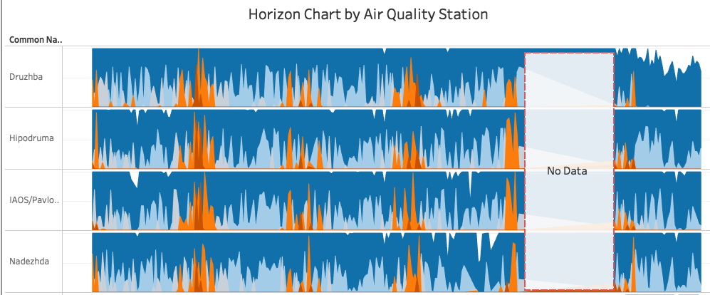
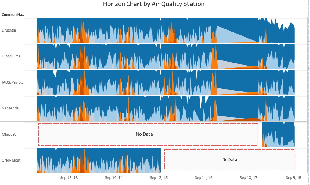
This issue crops up in two ways. Firstly, there is no air quality data recorded between 1st January 2017 and 27th November 2017. Secondly, Station Mladost only begins operation in December 2017, and Station Orlov Most ceased recording on the 27th of September 2017. | This issue crops up in two ways. Firstly, there is no air quality data recorded between 1st January 2017 and 27th November 2017. Secondly, Station Mladost only begins operation in December 2017, and Station Orlov Most ceased recording on the 27th of September 2017. | ||
| − | [[File:Screenshot 2018-11-18 at 10.56.05 PM.png| | + | [[File:Screenshot 2018-11-18 at 10.56.05 PM.png|frame|center]]] |
| − | [[File:Gaps in data.png| | + | [[File:Gaps in data.png|frame|center]]] |
<b>Solution 1. :</b> Account for Time-gaps in analysis </br> | <b>Solution 1. :</b> Account for Time-gaps in analysis </br> | ||
| Line 37: | Line 37: | ||
<b>Solution 2. :</b> Use "DateTime End" as a benchmark to standardise measurement validity </br> | <b>Solution 2. :</b> Use "DateTime End" as a benchmark to standardise measurement validity </br> | ||
| − | For our analysis, we will take that the air quality reading taken at 'var' times as representative of the entire hour before it's valdidity end time. Hence, we will create a new calculated field in tableau, that will deduct 1 hour, from the Datetime End field, which we will take to be the new start time. | + | For our analysis, we will take that the air quality reading taken at 'var' times as representative of the entire hour before it's valdidity end time. Hence, we will create a new calculated field in tableau, that will deduct 1 hour, from the Datetime End field, which we will take to be the new start time. |
| − | |||
===Citizen Science Air Quality Measurements=== | ===Citizen Science Air Quality Measurements=== | ||
| Line 51: | Line 50: | ||
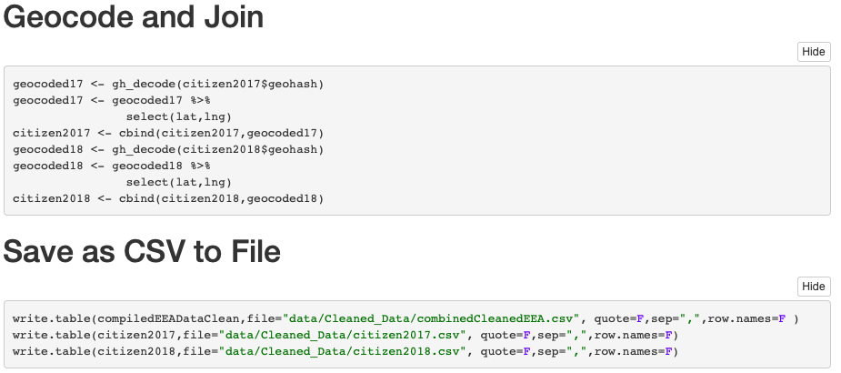
To obtain the latlng pair, we will have to rely on the R package "ironholds/geohash", which; while no longer maintained on CRAN, can be downloaded from github, with the devtools library. | To obtain the latlng pair, we will have to rely on the R package "ironholds/geohash", which; while no longer maintained on CRAN, can be downloaded from github, with the devtools library. | ||
| − | [[File:Screenshot 2018-11-18 at 10.27.22 PM.png| | + | [[File:Screenshot 2018-11-18 at 10.27.22 PM.png|frame|center]] |
We will then decode each geohash, and join it accordingly, with the R script below : | We will then decode each geohash, and join it accordingly, with the R script below : | ||
| − | [[File:Screenshot 2018-11-19 at 12.11.11 AM.png| | + | [[File:Screenshot 2018-11-19 at 12.11.11 AM.png|frame|center]] |
| − | |||
<b>Issue 2. :</b> Sensor Unreliability. </br> | <b>Issue 2. :</b> Sensor Unreliability. </br> | ||
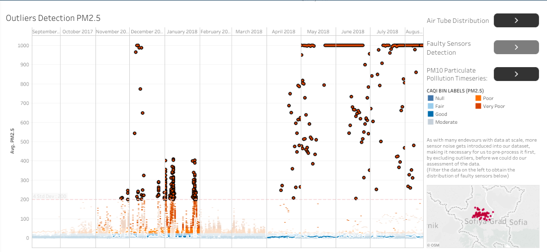
| − | With any crowdsourced sensor project, comes the possiblility that noise gets introduced into our dataset. In our case, noise seems to exhibit itself in the form of extreme outliers in our Air | + | With any crowdsourced sensor project, comes the possiblility that noise gets introduced into our dataset. In our case, noise seems to exhibit itself in the form of extreme outliers in our Air Quality readings. |
| − | |||
<b>Solution 2. :</b> Filter Outliers at 4 Std Dev. </br> | <b>Solution 2. :</b> Filter Outliers at 4 Std Dev. </br> | ||
| − | With Tableau, we will first create a reference line at the 4 Standard | + | With Tableau, we will first create a reference line at the 4 Standard Deviation Mark. Where the default practice would be to accept only data within the 3 Standard Deviations, the outliers here seem too extreme, and hence; we will choose to filter at 4 Std Dev instead. |
| − | + | [[File:Screenshot 2018-11-19 at 1.13.55 AM.png|frame|center]] | |
| − | |||
| + | From here, it's just an easy exclusion of selected data, which will apply to all sheets using the dataset. | ||
===Topographical Data=== | ===Topographical Data=== | ||
| Line 74: | Line 71: | ||
This dataset includes topographical data of Sophia Grad. From a quick visualisation of the data, it seems to cover only the city centre, and a small part of a neighbouring mountain. This confirms that the city lies at the foot of a mountain. | This dataset includes topographical data of Sophia Grad. From a quick visualisation of the data, it seems to cover only the city centre, and a small part of a neighbouring mountain. This confirms that the city lies at the foot of a mountain. | ||
| − | What the data does not show however, is that the city lies in a valley, an observation only made after having visualised the data with a Mapbox basemap, which gives us a larger context. | + | What the data does not show however, is that the city lies in a valley, an observation only made after having visualised the data with a Mapbox basemap, which gives us a larger context. |
| + | [[File:Screenshot 2018-11-18 at 10.39.08 PM.png|frame|center]] | ||
===Meteorological Data=== | ===Meteorological Data=== | ||
| Line 84: | Line 82: | ||
==Task 1: Spatio-temporal Analysis of Official Air Quality== | ==Task 1: Spatio-temporal Analysis of Official Air Quality== | ||
| − | + | <b> | |
| − | Characterize the past and most recent situation with respect to air quality measures in Sofia City. What does a typical day look like for Sofia city? | + | Characterize the past and most recent situation with respect to air quality measures in Sofia City. What does a typical day look like for Sofia city?</b> |
To answer this question, I have created a dashboard that expresses a calandar heatmap view of the PM10 Pollution density in Sophia Grad. From here, users can observe how the pollution levels change from month to month, and year to year. | To answer this question, I have created a dashboard that expresses a calandar heatmap view of the PM10 Pollution density in Sophia Grad. From here, users can observe how the pollution levels change from month to month, and year to year. | ||
One could also hover across dates between December 2017 and September 2018 to see how the pollution levels differ on an hourly basis. One can observe that PM10 levels spike at around 8AM, and between 7PM to 8PM. A measured difference that could be due to rush hour traffic. | One could also hover across dates between December 2017 and September 2018 to see how the pollution levels differ on an hourly basis. One can observe that PM10 levels spike at around 8AM, and between 7PM to 8PM. A measured difference that could be due to rush hour traffic. | ||
| + | [[File:Screenshot 2018-11-19 at 1.21.13 AM.png|frame]] | ||
| + | |||
| Line 95: | Line 95: | ||
The first and most obvious trend would be the seasonal nature of Air Pollution in Sophia Grad. | The first and most obvious trend would be the seasonal nature of Air Pollution in Sophia Grad. | ||
| + | |||
| + | [[File:Screenshot 2018-11-19 at 1.23.45 AM.png|frame]] | ||
From the cycle plot on the above, one can see clearly how seasonality plays a role in higher concentrations of PM10 particulate matter. PM10 ratings spike just as we hit the Winter months of the year, and decreases again as the weather warms again in the spring. | From the cycle plot on the above, one can see clearly how seasonality plays a role in higher concentrations of PM10 particulate matter. PM10 ratings spike just as we hit the Winter months of the year, and decreases again as the weather warms again in the spring. | ||
| Line 110: | Line 112: | ||
When visualising the data, it would be important to leave obvious annotations to mark where data has been missing, so users can assess it accordingly. | When visualising the data, it would be important to leave obvious annotations to mark where data has been missing, so users can assess it accordingly. | ||
| − | + | [[File:Gaps in data.png|frame]] | |
| − | |||
| − | |||
| + | Since data is missing, we cannot correctly access the aggregate PM10 concentration levels of 2017, or 2018, because both datasets are incomplete in time periods, and as previously mentioned, are highly seasonal, both 2017 and 2018 are missing half a winter season each. | ||
==Task 2: Spatio-temporal Analysis of Citizen Science Air Quality Measurements == | ==Task 2: Spatio-temporal Analysis of Citizen Science Air Quality Measurements == | ||
| Line 121: | Line 122: | ||
<b>Characterize the sensors’ coverage, performance and operation. Are they well distributed over the entire city?</b> | <b>Characterize the sensors’ coverage, performance and operation. Are they well distributed over the entire city?</b> | ||
| + | [[File:Screenshot 2018-11-18 at 11.34.52 PM.png|center|thumb]] | ||
The distribution of sensors are mainly centred around the city centre, and starts to spread out in to the periphery from the start of 2018. This network of air quality sensors, while well distributed among populated areas, do not cover yet cover more rural areas, or national parks, and hence may create a bias towards city centres and suburban areas. | The distribution of sensors are mainly centred around the city centre, and starts to spread out in to the periphery from the start of 2018. This network of air quality sensors, while well distributed among populated areas, do not cover yet cover more rural areas, or national parks, and hence may create a bias towards city centres and suburban areas. | ||
| Line 126: | Line 128: | ||
<b>Do the sensors work all the time?</b> | <b>Do the sensors work all the time?</b> | ||
| + | [[File:Screenshot 2018-11-18 at 11.18.58 PM.png|center|thumb|Oct 2017]] | ||
No, there are periods, such as on the 10th of October 2017 and the 15th of November 2017, where all the sensors will all stop recording for a few hours, before going back on again. This could be due to a server patch, or maintenance, but we can only speculate at this point. | No, there are periods, such as on the 10th of October 2017 and the 15th of November 2017, where all the sensors will all stop recording for a few hours, before going back on again. This could be due to a server patch, or maintenance, but we can only speculate at this point. | ||
| Line 131: | Line 134: | ||
<b>Can you detect any unexpected behaviors of the sensors through analyzing the readings they capture? </b> | <b>Can you detect any unexpected behaviors of the sensors through analyzing the readings they capture? </b> | ||
| − | As previously mentioned, there are a couple of known sensors that | + | As previously mentioned, there are a couple of known sensors that consistently report extreme outliers, which we will exclude from our analysis. |
| − | |||
| − | |||
| Line 139: | Line 140: | ||
Which part of the city shows relatively higher readings than others? </b> | Which part of the city shows relatively higher readings than others? </b> | ||
| + | [[File:Screenshot 2018-11-19 at 1.40.58 AM.png|center|frame]] | ||
The city centre happens to measure with the highest readings in Sophia Grad. This is unsurprising, as the city is dense with road networks, which presumably carry traffic that will emit the types of particulates accounted for in the PM10 to PM2.5 range. | The city centre happens to measure with the highest readings in Sophia Grad. This is unsurprising, as the city is dense with road networks, which presumably carry traffic that will emit the types of particulates accounted for in the PM10 to PM2.5 range. | ||
| + | [[File:Screenshot 2018-11-18 at 11.37.15 PM.png|center|thumb]] | ||
| + | [[File:Screenshot 2018-11-18 at 11.25.50 PM.png|thumb|center]] | ||
One surprising spot for high PM10 density happens to be around the vicinity of the Rakovski Defence and Staff Collage, which happens to also have a dense road network, even with a couple of metro stations in the vicinity. | One surprising spot for high PM10 density happens to be around the vicinity of the Rakovski Defence and Staff Collage, which happens to also have a dense road network, even with a couple of metro stations in the vicinity. | ||
| Line 148: | Line 152: | ||
The data captured by the citizens of Sophia Grad happens to closely mirror the patterns tracked by official air measurements. | The data captured by the citizens of Sophia Grad happens to closely mirror the patterns tracked by official air measurements. | ||
| − | Likewise, Seasonality plays a major role in the PM10 density levels of the the city. The winter months between November till | + | [[File:Screenshot 2018-11-18 at 11.48.40 PM.png|frame|center]] |
| − | + | Likewise, Seasonality plays a major role in the PM10 density levels of the the city. The winter months between November till February will see spikes in PM10 Concentration levels, with the worst month of the pollution happening in January. | |
| − | |||
| − | |||
==Task 3== | ==Task 3== | ||
| Line 166: | Line 168: | ||
| + | [[File:Screenshot 2018-11-19 at 1.52.43 AM.png|frame|center]] | ||
Given that Sofia Grad lies in a valley, it is no wonder that the city is plauged by heavy particulate pollution each winter. Cold, dense air tends to cause particles to be less likely to react with the water mollucules in the air, causing it to linger in the atmosphere. | Given that Sofia Grad lies in a valley, it is no wonder that the city is plauged by heavy particulate pollution each winter. Cold, dense air tends to cause particles to be less likely to react with the water mollucules in the air, causing it to linger in the atmosphere. | ||
The correlation matrix on the far left confirms this theory, showing dew point average, and tempreture to be negatively correlated to PM10 density, while humidity is positively correlated to PM10 density. Likewise, it also shows that Wind is negatively correlated to PM10 density, which could indicate that there might be a leak-on effect of air pollution to cities neighbouring Sofia Grad. | The correlation matrix on the far left confirms this theory, showing dew point average, and tempreture to be negatively correlated to PM10 density, while humidity is positively correlated to PM10 density. Likewise, it also shows that Wind is negatively correlated to PM10 density, which could indicate that there might be a leak-on effect of air pollution to cities neighbouring Sofia Grad. | ||
| − | |||
| − | |||
| − | |||
| − | |||
| − | |||
| − | |||
| − | |||
=References= | =References= | ||
Latest revision as of 01:55, 19 November 2018
Contents
Overview
Air pollution is an important risk factor for health in Europe and worldwide. A recent review of the global burden of disease showed that it is one of the top ten risk factors for health globally. Worldwide an estimated 7 million people died prematurely because of pollution; in the European Union (EU) 400,000 people suffer a premature death. The Organisation for Economic Cooperation and Development (OECD) predicts that in 2050 outdoor air pollution will be the top cause of environmentally related deaths worldwide. In addition, air pollution has also been classified as the leading environmental cause of cancer.
Air quality in Bulgaria is a big concern: measurements show that citizens all over the country breathe in air that is considered harmful to health. For example, concentrations of PM2.5 and PM10 are much higher than what the EU and the World Health Organization (WHO) have set to protect health.
Bulgaria had the highest PM2.5 concentrations of all EU-28 member states in urban areas over a three-year average. For PM10, Bulgaria is also leading on the top polluted countries with 77 μg/m3on the daily mean concentration (EU limit value is 50 μg/m3).
According to the WHO, 60 percent of the urban population in Bulgaria is exposed to dangerous (unhealthy) levels of particulate matter (PM10).
Tableau Public Dashboard : https://public.tableau.com/profile/sean.koh6959#!/vizhome/Sean_Koh_2015_VA_Assignment/Dashboard1-1?publish=yes
Data Exploration
Official Air Quality Dataset
This would be the official Air Quality Reading taken from EEA, which covers the timeperiods between January 2013 till September 2018. One particularity of this dataset is that readings are not performed hourly, till the December of 2017. This does not invalidate the dataset, but should be considered, alongside the following issues :
Issue 1. : Time gaps where no data is collected.
This issue crops up in two ways. Firstly, there is no air quality data recorded between 1st January 2017 and 27th November 2017. Secondly, Station Mladost only begins operation in December 2017, and Station Orlov Most ceased recording on the 27th of September 2017.
]
]
Solution 1. : Account for Time-gaps in analysis
For these periods in time, we just have no way to account for, and as there is no ready solution for it, we will have to simply account for these gaps in our analysis.
Issue 2. : Variable Recording Timings.
Air Quality Recordings are not always taken at a single starndard start time, but are always valid till specific end timings, which are at scheduled hourly intervals. Hence, a single reading could either represent an hour of a day, a whole day, or at 'variable' or 'var' times of a day.
Solution 2. : Use "DateTime End" as a benchmark to standardise measurement validity
For our analysis, we will take that the air quality reading taken at 'var' times as representative of the entire hour before it's valdidity end time. Hence, we will create a new calculated field in tableau, that will deduct 1 hour, from the Datetime End field, which we will take to be the new start time.
Citizen Science Air Quality Measurements
These are datasets gathered by the citizens of Sophia Grad. Allowing us a higher granularity and coverage of the air quality in the city.
Issue 1. : Geohashed Coordinates.
Unlike the official data which comes with a latlng pair for each station in the metadata, each AirTube record comes with a Geohash, which we will have to decode on our own, do obtain a latlng pair.
Solution 1. : Decode with an R Library.
To obtain the latlng pair, we will have to rely on the R package "ironholds/geohash", which; while no longer maintained on CRAN, can be downloaded from github, with the devtools library.
We will then decode each geohash, and join it accordingly, with the R script below :
Issue 2. : Sensor Unreliability.
With any crowdsourced sensor project, comes the possiblility that noise gets introduced into our dataset. In our case, noise seems to exhibit itself in the form of extreme outliers in our Air Quality readings.
Solution 2. : Filter Outliers at 4 Std Dev.
With Tableau, we will first create a reference line at the 4 Standard Deviation Mark. Where the default practice would be to accept only data within the 3 Standard Deviations, the outliers here seem too extreme, and hence; we will choose to filter at 4 Std Dev instead.
From here, it's just an easy exclusion of selected data, which will apply to all sheets using the dataset.
Topographical Data
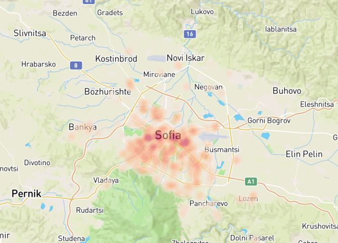
This dataset includes topographical data of Sophia Grad. From a quick visualisation of the data, it seems to cover only the city centre, and a small part of a neighbouring mountain. This confirms that the city lies at the foot of a mountain.
What the data does not show however, is that the city lies in a valley, an observation only made after having visualised the data with a Mapbox basemap, which gives us a larger context.
Meteorological Data
Contains the daily recordings of Temperature; Humidity; Wind speed; Pressure; Rainfall; Visibility in Sophia Grad. This will be useful later when drawing correlations between these Meteorological elements, and Pollution Density.
Task 1: Spatio-temporal Analysis of Official Air Quality
Characterize the past and most recent situation with respect to air quality measures in Sofia City. What does a typical day look like for Sofia city?
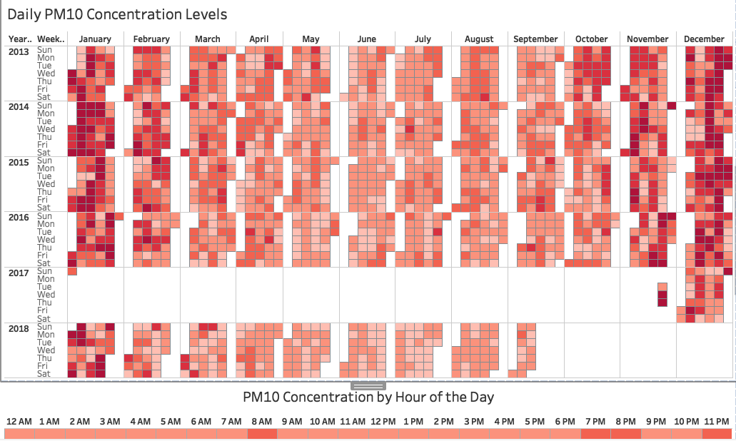
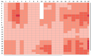
To answer this question, I have created a dashboard that expresses a calandar heatmap view of the PM10 Pollution density in Sophia Grad. From here, users can observe how the pollution levels change from month to month, and year to year.
One could also hover across dates between December 2017 and September 2018 to see how the pollution levels differ on an hourly basis. One can observe that PM10 levels spike at around 8AM, and between 7PM to 8PM. A measured difference that could be due to rush hour traffic.
Do you see any trends of possible interest in this investigation?
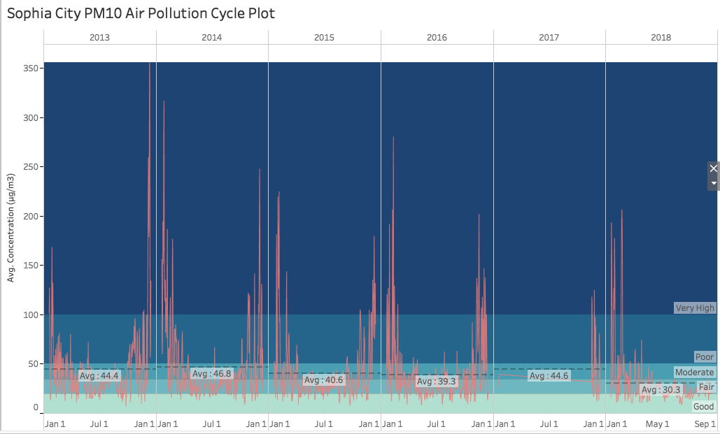
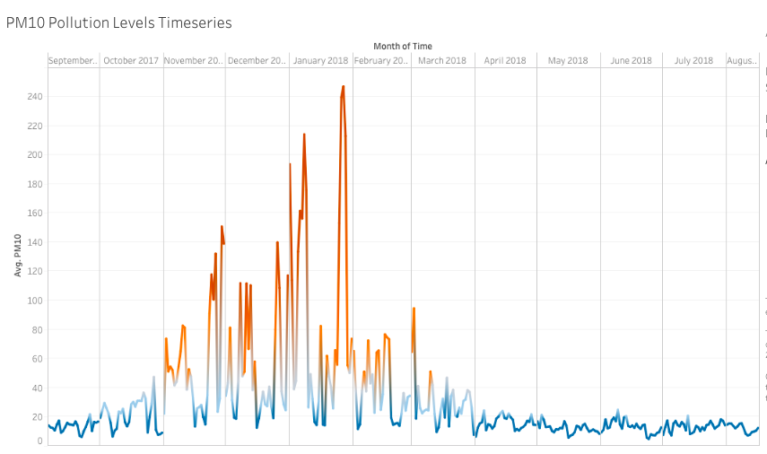
The first and most obvious trend would be the seasonal nature of Air Pollution in Sophia Grad.
From the cycle plot on the above, one can see clearly how seasonality plays a role in higher concentrations of PM10 particulate matter. PM10 ratings spike just as we hit the Winter months of the year, and decreases again as the weather warms again in the spring.
The Average PM10 levels happen to fall between the Moderate and Fair levels each year, and while the average for 2018 has been the lowest thus far, we have not yet accounted for the winter months of 2018.
What anomalies do you find in the official air quality dataset?
As aforementioned, there are gaps in the official air quality dataset, and that has been addressed in the "issues" portions of the exploratory data analysis.
How do these affect your analysis of potential problems to the environment?
When visualising the data, it would be important to leave obvious annotations to mark where data has been missing, so users can assess it accordingly.
Since data is missing, we cannot correctly access the aggregate PM10 concentration levels of 2017, or 2018, because both datasets are incomplete in time periods, and as previously mentioned, are highly seasonal, both 2017 and 2018 are missing half a winter season each.
Task 2: Spatio-temporal Analysis of Citizen Science Air Quality Measurements
Using appropriate data visualisation, you are required will be asked to answer the following types of questions:
Characterize the sensors’ coverage, performance and operation. Are they well distributed over the entire city?
The distribution of sensors are mainly centred around the city centre, and starts to spread out in to the periphery from the start of 2018. This network of air quality sensors, while well distributed among populated areas, do not cover yet cover more rural areas, or national parks, and hence may create a bias towards city centres and suburban areas.
Do the sensors work all the time?
No, there are periods, such as on the 10th of October 2017 and the 15th of November 2017, where all the sensors will all stop recording for a few hours, before going back on again. This could be due to a server patch, or maintenance, but we can only speculate at this point.
Can you detect any unexpected behaviors of the sensors through analyzing the readings they capture?
As previously mentioned, there are a couple of known sensors that consistently report extreme outliers, which we will exclude from our analysis.
Now turn your attention to the air pollution measurements themselves.
Which part of the city shows relatively higher readings than others?
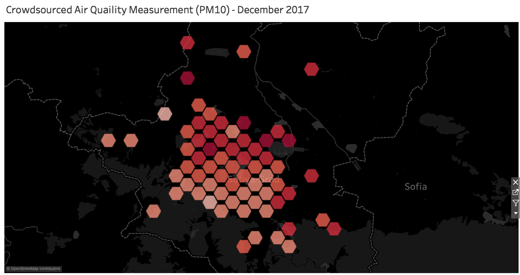
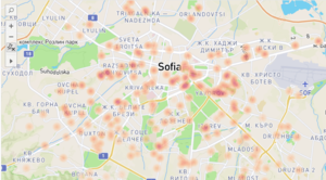
The city centre happens to measure with the highest readings in Sophia Grad. This is unsurprising, as the city is dense with road networks, which presumably carry traffic that will emit the types of particulates accounted for in the PM10 to PM2.5 range.
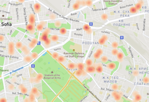
One surprising spot for high PM10 density happens to be around the vicinity of the Rakovski Defence and Staff Collage, which happens to also have a dense road network, even with a couple of metro stations in the vicinity.
Are these differences time dependent?
The data captured by the citizens of Sophia Grad happens to closely mirror the patterns tracked by official air measurements.
Likewise, Seasonality plays a major role in the PM10 density levels of the the city. The winter months between November till February will see spikes in PM10 Concentration levels, with the worst month of the pollution happening in January.
Task 3
Urban air pollution is a complex issue. There are many factors affecting the air quality of a city. Some of the possible causes are:
- Local energy sources. For example, according to Unmask My City, a global initiative by doctors, nurses, public health practitioners, and allied health professionals dedicated to improving air quality and reducing emissions in our cities, Bulgaria’s main sources of PM10, and fine particle pollution PM2.5 (particles 2.5 microns or smaller) are household burning of fossil fuels or biomass, and transport.
- Local meteorology such as temperature, pressure, rainfall, humidity, wind etc
- Local topography
- Complex interactions between local topography and meteorological characteristics.
- Transboundary pollution for example the haze that intruded into Singapore from our neighbours.
Reveal the relationships between the factors mentioned above and the air quality measure detected in Task 1 and Task 2.
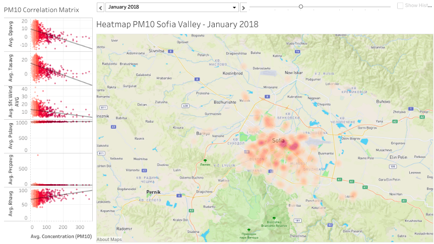
Given that Sofia Grad lies in a valley, it is no wonder that the city is plauged by heavy particulate pollution each winter. Cold, dense air tends to cause particles to be less likely to react with the water mollucules in the air, causing it to linger in the atmosphere.
The correlation matrix on the far left confirms this theory, showing dew point average, and tempreture to be negatively correlated to PM10 density, while humidity is positively correlated to PM10 density. Likewise, it also shows that Wind is negatively correlated to PM10 density, which could indicate that there might be a leak-on effect of air pollution to cities neighbouring Sofia Grad.
References
1. Air pollution in the Winter : https://www.futurity.org/winter-air-pollution-emissions-1819872/
2. Air Quality Index :
https://www.eea.europa.eu/themes/air/air-quality-index/index#tab-based-on-data
