IS428 AY2018-19T1 Zhuo Yunying

Problem & Motivation

Air pollution is an important risk factor for health in Europe and worldwide. A recent review of the global burden of disease showed that it is one of the top ten risk factors for health globally. Worldwide an estimated 7 million people died prematurely because of pollution; in the European Union (EU) 400,000 people suffer a premature death. The Organisation for Economic Cooperation and Development (OECD) predicts that in 2050 outdoor air pollution will be the top cause of environmentally related deaths worldwide. In addition, air pollution has also been classified as the leading environmental cause of cancer. Air quality in Bulgaria is a big concern: measurements show that citizens all over the country breathe in air that is considered harmful to health. For example, concentrations of PM2.5 and PM10 are much higher than what the EU and the World Health Organization (WHO) have set to protect health. Bulgaria had the highest PM2.5 concentrations of all EU-28 member states in urban areas over a three-year average. For PM10, Bulgaria is also leading on the top polluted countries with 77 μg/m3on the daily mean concentration (EU limit value is 50 μg/m3).According to the WHO, 60 percent of the urban population in Bulgaria is exposed to dangerous (unhealthy) levels of particulate matter (PM10).

This assignment aims to study the following:

• Task 1: Spatio-temporal Analysis of Official Air Quality
• Task 2: Spatio-temporal Analysis of Citizen Science Air Quality Measurements
• Task 3: Find out the relationship of the above analysis with other factors (Local energy sources, Local meteorology, Local topography, Complex interactions between local topography and meteorological characteristics and Transboundary pollution)

Dataset Analysis & Transformation Process

1. Combine all time-series data (e.g. BG_5_9572_2017_timeseries) into one single excel spreadsheet

• • Create a new "Station" Column (indicating station code i.e. 9421) and "Year" Column based on the year for each of the time-series data
  • Use excel to combine the rest of time-series files based on all the common columns (e.g. Countrycode, Namespace, AirQualityNetwork and etc.)
  • Based on the analysis of the existing combined time-series data from 2013 to 2018, there is a drastic difference in the level of aggregation across the years. As shown in the table below, Year 2016 has a combination of hourly air quality readings and daily air quality readings while in 2017, there is a mixture of hour and var readings as for certain days, readings are not measured at one-hour interval continuously. As such, the analysis on air quality readings will be based on "Day" averaging time from year 2013 to 2016 as it is impossible to lower the aggregation level of "Day" to "Hour" readings in 2016. On the other hand, the analysis on air quality readings will be based on "Hour" averaging time for 2017 and 2018. For the data in 2017, average readings will be taken if the readings for any specific days are done on "Var" basis.

• • Due to the standardization in averaging time, the values under "Concentration", "DatetimeBegin" and "DatetimeEnd" have been adjusted accordingly while other column values remain unchanged.
  • There are quite a number of duplicated readings in the dataset. These duplicated readings are removed during the transformation process to avoid unequal weightage.
  • Due to the high variation in raw data and small dataset, excel is used for the transformation process.

2. Merge metadata file with combined time-series data

• • According to the source of scrapped data (http://discomap.eea.europa.eu/map/fme/AirQualityExport.htm), "the join between time-series files and the metadata file should be made using the Countrycode (or Namespace) and SamplingPoint". Thus, metadata file and time-series data time are merged via Vlookup function in excel based on SamplingPoint (since Countrycode are all "BA" for both data file).
  • Upon further inspection, these two datasets have a number of common columns with same values. These columns include "Countrycode, Namespace, AirQualityNetwork, AirQualityStation, AirQualityStationEoICode, SamplingProcess, AirPollutantCode, AirPollutant" and thus repeated columns are removed.

Task 2: Spatio-temporal Analysis of Official Air Quality

Geohash tells the station locations. However Tableau is not able to interpret geohash as geographic data. Before Air Tube data is imported to Tableau for analysis, geohash needs to be decoded into geographical coordinates. As the two Air Tube data files- data_bg_2017.xlsx and data_bg_2018.xlsx are of big sizes and there are duplicate geohash records in the data, an Excel file containing a unique geohash list was created.

Step 1: Use "pygeohash" package to decode the geohash list and output the coordinates in an Excel file

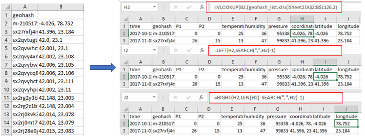
Step 2: Combine geohash list and coordinates list into one Excel file and update the coordinates, latitude, longitude in data_bg_2017.xlsx and data_bg_2018.xlsx using VLOOKUP, LEFT and RIGHT functions in Excel

Decode the geohash column in Air Tube data files

Geohash tells the station locations. However Tableau is not able to interpret geohash as geographic data. Before Air Tube data is imported to Tableau for analysis, geohash needs to be decoded into geographical coordinates. As the two Air Tube data files- data_bg_2017.xlsx and data_bg_2018.xlsx are of big sizes and there are duplicate geohash records in the data, an Excel file containing a unique geohash list was created.

Step 1: Use "pygeohash" package to decode the geohash list and output the coordinates in an Excel file

Step 2: Combine geohash list and coordinates list into one Excel file and update the coordinates, latitude, longitude in data_bg_2017.xlsx and data_bg_2018.xlsx using VLOOKUP, LEFT and RIGHT functions in Excel

Combine multiple yearly data files into one time series data file

Dataset Import Structure & Process

Datasets Imported to Tableau for Analysis

• Air Tube datasets with geohash column being decoded
• EEA time series data

• EEA metadata to show station locations
• METEO-data
• TOPO-data

Join METEO-Data and Station STA-BG0052A Timeseries Data

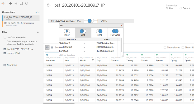
With the given Meteo-data, which describes the temerature, wind speed, humidity, pressure and rainfall in Sofia Airport (42.6537, 23.3829 ), we can investigate the relationships between meteorology and air pollution. Since station STA-BG0052A(42.6665, 23.4002) is closest to Sofia Airport compared with other three stations, I use data in station STA-BG0052A for Comparison. Before visualising the two datasets, it is better to join them into one dataset. This can be done in tableau.

The two datasets was joined by dates. Since the dates in the Meteo-data file are separate into year, month and day and the data types are string. Before joining them, the data types need to be changed to date.

Interactive Visualization

The interactive visualization can be accessed here: https://public.tableau.com/profile/fu.yu#!/vizhome/AirQualityinBulgaria/Story1?publish=yes

Official Air Quality in Sofia City

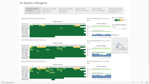
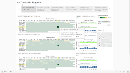
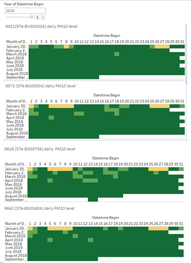
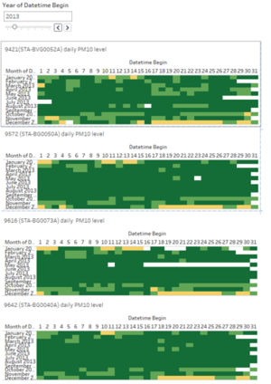
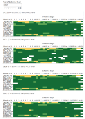
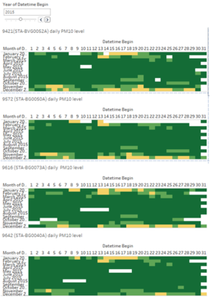
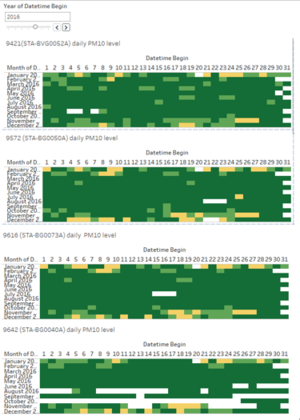
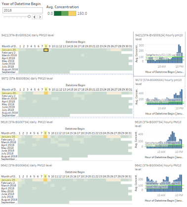
This dashboard shows the daily and hourly PM10 concentration in the 4 measured stations. A user can select a day on the heat map and investigate PM10 concentration at different times of the day.

Sensor Coverage, Performance and Operation

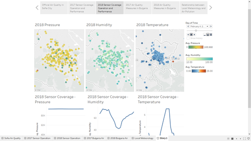
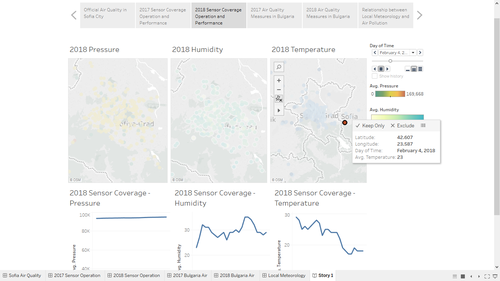
This dashboard shows sensors and their readings in Sofia City. When selecting a sensor, the line charts will display the sensor readings at different times of the day. A user thus can tell when the sensors start not working properly.

Air Quality Measures in Sofia City

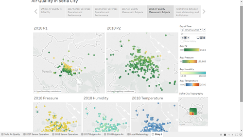
This dashboard helps user see the flow of air pollution from day to day and analyse the impacts of local topography and meteorology on air quality.

Relationship between Local Meteorology and Air Pollution

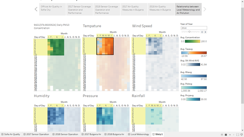
The last dashboard helps user find the relationship between local meteorology and air pollution. A user can select a few days and compare the patterns among temperature, pressure, rainfall, humidity, wind and air quality.

Interesting & Anomalous Observations

Task 1: Spatio-temporal Analysis of Official Air Quality

1.1 Most Recent and Past Situation of Air Quality in Sofia City The above graphs display the PM10 concentration in Sofia City from January 2013 to September 2018 where data for 2017 is omitted because there is only November and December data. Dark green indicates good air quality where PM10 concentration <= 50 ug/m3 . Light green indicates satisfactory air quality where 51 ug/m3 < PM10 concentration <=100 ug/m3. Yellow indicates poor air quality where PM10 concentration > 100 ug/m3. Each heatmap represents the air quality of one measured station in Sofia City. Trends: Air quality in all the four stations is usually poor at the start and the end of a year. Being the station with fewest days having good air quality in 2013, station STA-BG0052A has the most days with good air quality in 2018 compared with other stations.

1.2 A Typical Day in Sofia City To investigate how PM10 concentrations vary from hours to hours in a day, one can simply highlight a day on the heatmap and the hourly PM10 concentration graphs will update accordingly. For example, as shown in the diagram above, on 8 January 2018, air quality in stations STA-BG0052A and STA-BG0050A is poor after 10pm while air quality in station STA-BG0073A is poor starting from 12pm and in STA-BG0040A, air quality is poor throughout the day. Trends: There is no obvious trend showing on what time of a day the PM10 concentration is higher or lower Nevertheless, PM10 concentrations do vary from time to time in a day.

1.3 Anomalies in the Datesetss From 2013 to 2015, hourly PM10 concentration data is not available. Data was either only collected at 00:00 once or the hour when the data was collected was not recorded from 2013 to 2015. Also, in 2016, data was only collected at 00:00 on some days. If the data was only collected at 00:00 or only collected once, it might affect the accuracy of PM10 concentration distribution across the year because PM10 concentrations are different at different time in a day. It might happen that at the time the data was collected, the PM10 concentration was too high or too low, which would not be representative of the PM10 concentration of a day. For 2017, only November and December data is available. Hence changes in air quality from 2016 to 2017 could not be investigated which might give the insights of why air quality in 2018 has improved.

Task 2: Spatio-temporal Analysis of Citizen Science Air Quality Measurements

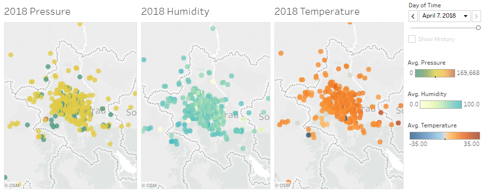
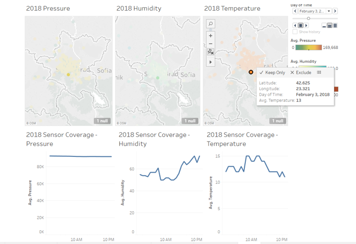
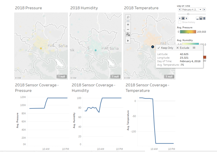
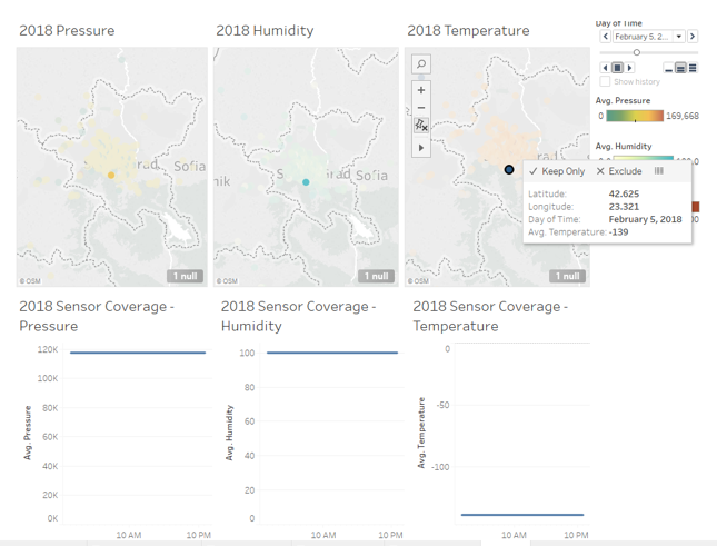
2.1 Sensor Coverage, Performance and Operation 2.1.1 Sensor Coverage The most recent sensor distribution (on 7 April 2018) shows that the sensors are not evenly spread out across the entire city. They are saturated in the center of the city. Nevertheless, the sensors did cover the central part of the city well. 2.1.2 Sensor Performance and Operation However, the sensors were not always working properly. As shown in the graphs above, fora example, on 3 February 2018, the sensor at (42.625, 23.321) was working properly. Its readings of pressure, humidity and temperature fluctuate within reasonable ranges though the day. However, on 4 February 2018, the sensor temperature reading had a sharp drop from 7 degree to -139 degree at 9AM, which is not reasonable. At the same time, pressure and humidity readings also increased sharply, suggesting that the sensor might have a problem on 9AM, 4 February 2018. The suspect was approved by the static sensor readings on 5 February 2018, suggesting that the sensor was not working. Similar sensor behaviors can also be seen on other sensors such as the sensor located at (42.686, 23.347) after 14 February 2018 and the sensor located at (42.715, 23.161) after 7 February 2018.

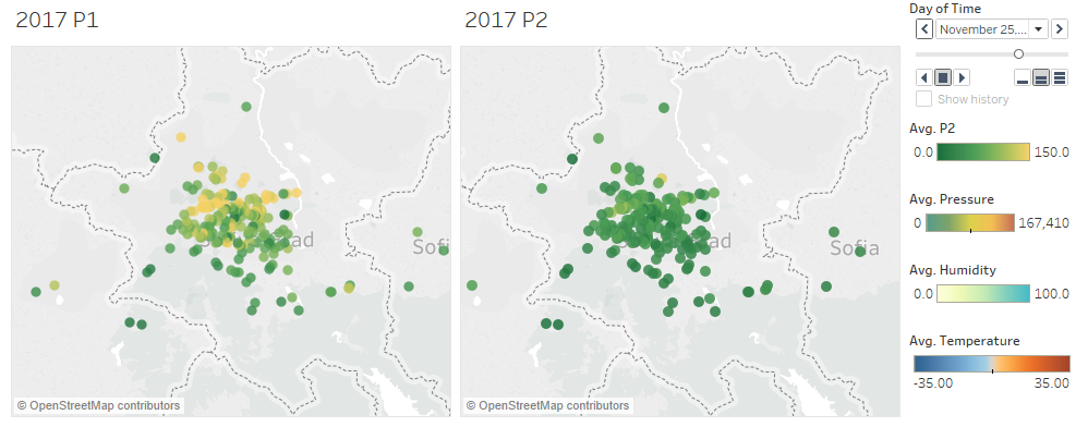
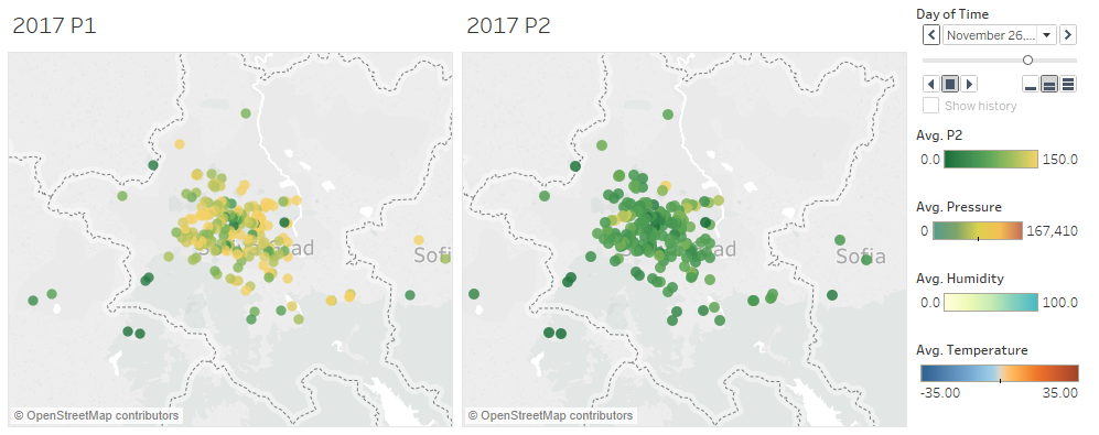
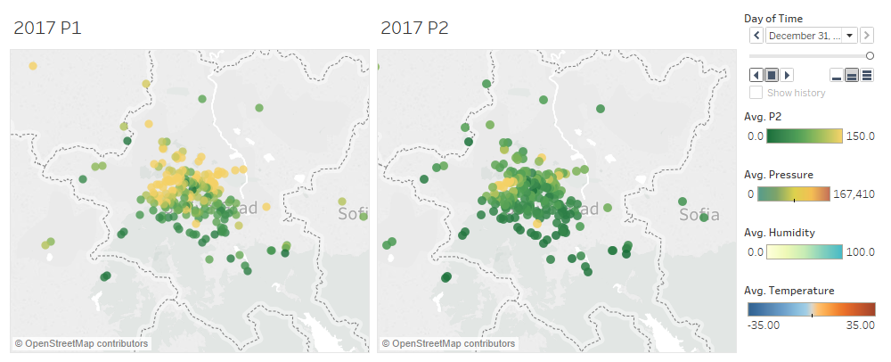
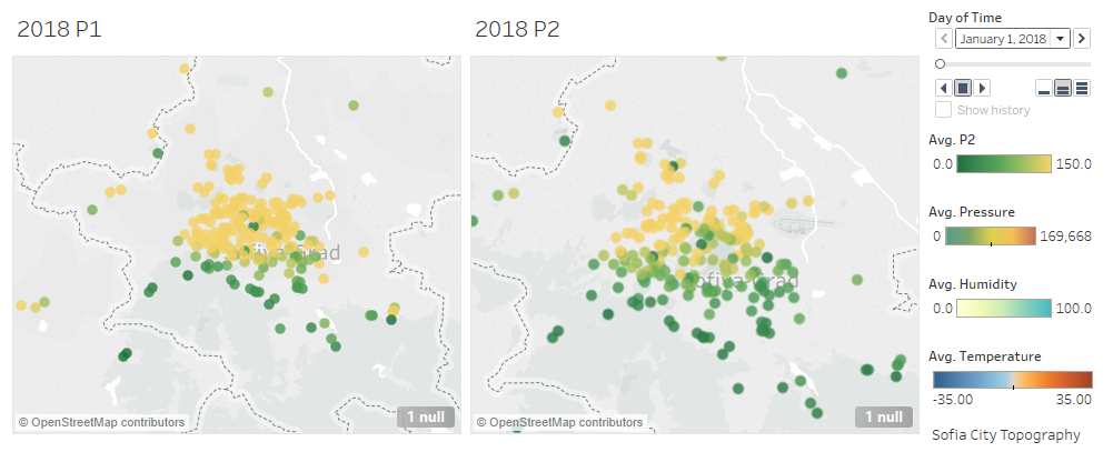
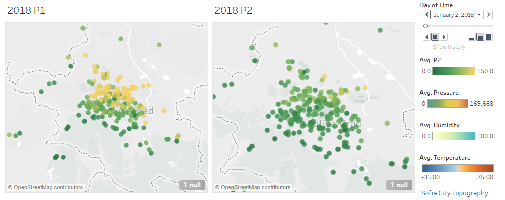
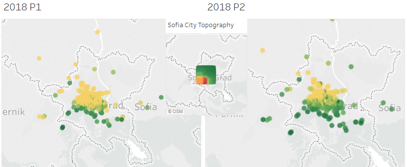
2.2 Air Pollution Most of the time, pollution started from the northern part of the city. As time passes, the pollution can spread in different directions. Case 1: Pollution spread to the south Case 2: Pollution spread to the south first and then back to the north

Task 3: Factors Affecting Air Quality in Sofia City

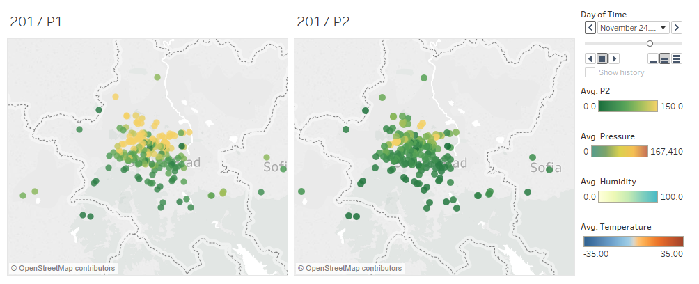
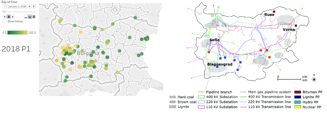
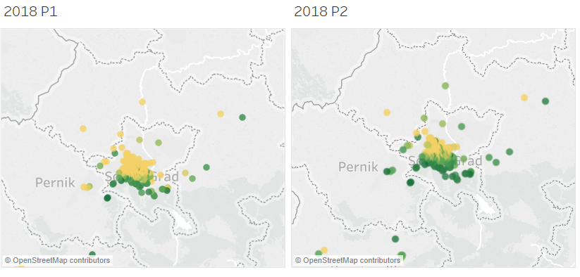
Factor 1: Local Energy Sources The diagrams above shows that in cities like Sofia and Blagoevgrad, P1 concentration is relatively high. This might be because these cities are along the main gas pipeline system. Since the cities are rich in hard coal, the gas and energy generated in these cities might be from burning of hard coals, which damages the air.

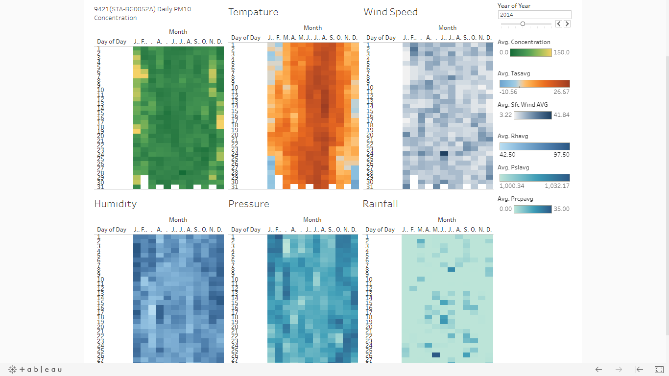
Factor 2: Local Meteorology With the given Meteo-data, which describes the temperature, wind speed, humidity, pressure and rainfall in Sofia Airport (42.6537, 23.3829 ), we can investigate the relationships between meteorology and air pollution. Since station STA-BG0052A(42.6665, 23.4002) is closest to Sofia Airport compared with other three stations, I use data in station STA-BG0052A for comparison. The diagrams above compare the patterns of temperature, wind speed, humidity, pressure and rainfall in Sofia Airport (42.6537, 23.3829 ) with the pattern of PM10 concentration in Station STA-BG0052A(42.6665, 23.4002) in 2014. It shows that PM10 concentration tends to be high in a low temperature, low wind speed, high humidity and high pressure environment. However, the relationship between rainfall and PM10 concentration is not very obvious. Data in 2016 also shows the same findings.

Factor 3: Local Topography As mentioned in Task 2, pollution usually starts from the northern part of Sofia city. This may be due to the fact that Sofia's altitude is low in the north and high in the southwest. PM10 particles from the north can flow into Sofia city much more easily than those from the southwest.

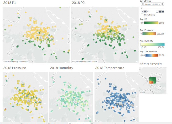
Factor 4: Complex interactions between local topography and meteorological characteristics The diagram shows that even though the pressure was high, humidity was high and temperature was low across the city, the pollution level is high in the northern part of the city mainly because of the low altitude in the northern part.

Factor 5: Transboundary Pollution Pollution does spread from one place to another as discussed in Task 2. The graph below also displays that when air quality in Sofia is poor, the cities around it also have places with poor air quality.

References

Understanding Particulate Matter and How It Impacts Our Health https://www.airveda.com/blog/Understanding-Particulate-Matter-and-Its-Associated-Health-Impact

Map on the Bulgarian Coal Resources and Energy Infrastructure https://www.researchgate.net/figure/Map-on-the-Bulgarian-coal-resources-energy-infrastructure-and-largest-power-plants_fig1_257941554

• https://www.eea.europa.eu/publications/air-quality-in-europe-2018/at_download/file