Assign Preparations
|
|
|
|
|
|
|
Contents
Data Manipulations
About the Dataset
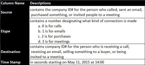
The insider has provided us with 10 datasets consisted of 4 files (calls, emails, meetings, purchases) with daily connections records among every staff in Kasios from year 2015 to year 2017, 5 files of suspicious records relative to each connections channels, and 1 file that has revealed all the staff ID in Kasios. And there is also a letter from the insider, that has revealed another group of people that he (she) thinks to be involved which may need further investigations. All connections data are in the same format as decriptions below:
It's made up by 4 columns with source, connection type that was designated by number, destination and time stamp. Data needs to be further formatted because there is no title, and timestamps are seconds counted from may 11, 2015 at 14:00. All connection types will union so that all interactions can be captured. All data manipulations were done in R.
Packages
- Package anytime will cast strings into parsed date or datetime, so that we will be able add seconds to timestamp and get exact date time.
- Package dplyr and tidyr will give us options for data manipulations like mutate, select and etc..
 library(tidyverse)
 library(knitr)
 library(readr)
 library(anytime)   # For time formating
 library(dplyr)  # For data manipulations
 library(tidyr)  # For data manipulations
Import Data
- Daily connection records
# ALL source files calls.csv, emails.csv, meetings.csv and purchases.csv have been loaded into the workspace
 # Union all sources and drop original column 'timestamp'
 sources <- select(mutate(rbind(calls, emails, meetings, purchases),
                          DT = anytime("2015-05-11 14:00:00") + Timestamp)
                   ,c(1,2,3,5))
- Suspicious Connections Records
Same formatting has also been done to suspicious connections lists. As a result, all connections from suspected staffs can be filtered out. This filtered dataset can be used as a breaking point for analysing suspected staffs.
 # Suspucious
 sps <- rbind(read.csv("MC3/Suspicious_calls.csv",header = FALSE),
              read.csv("MC3/Suspicious_emails.csv",header = FALSE),
              read.csv("MC3/Suspicious_meetings.csv",header = FALSE),
              read.csv("MC3/Suspicious_purchases.csv",header = FALSE))
 colnames(sps) <- c("Source","Etype","Destination","Timestamp")
       # Format Datetime
 sps <- mutate(sps, DT = anytime("2015-05-11 14:00:00") + Timestamp)
 sps <- select(sps, c(1,2,3,5))
 # filter only suspicious staff from source file
 sps_list <- unique(rbind(sps$Source,sps$Destination))
 filter_sps <- rbind(subset(sources, Source %in% sps_list),
                     subset(sources, Destination %in% sps_list))
 # Summarise suspicios connections
 filter_sps %>%
     group_by(as.factor(filter_sps$Etype)) %>%
     summarise(count = n())
In the filtered connection dataset of suspected staffs, 945 records are from calls, 1,179 records come from emails.
Data Aggregation
To monitor the company’s communication habits, patterns of communications need to be analysed. The original 4 datasets contain millions of records, which has made it very difficult to extract useful information. Thus, some data aggregations were required.
All records were grouped by date, and connection type. Values are filled by frequency.
 # Seperate timestamp column into 2 to get date informaion
 sources <- sources %>%
            separate(DT, c("date","time"), sep = " " )
 agg_data <- sources %>%
             group_by(date, Etype) %>%
             summarize(count=n())
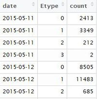
The aggregate data format looks like something below. The aggregated data can then be imported into tableau for visual explorations.
Preparing Data for Network Explorations
for network analysis part, we will also need information for staff name correspondent to their staff IDs. Thus, staffs who are listed in supspected list can be extracted from company index.
 nodes <- read.csv("MC3/CompanyIndex.csv")
   # combine first and last name columns for full name
   nodes <- unite(nodes, Name, c(first,last), sep = '.', remove = TRUE)
   # filter nodes based on suspected list above
   filter_nodes <- subset(nodes, ID %in% sps_list)
Summary
With all the efforts above, we now have couple sets of data that can be used for analysis. They can be summarized as below:


