ISSS608 2017-18 T3 Assign Low Zhi Wei Methodology
Contents
Approach
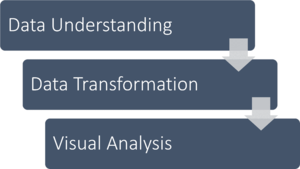
The approach to this exercise is captured in the flow below. Unlike in most typical data analysis undertakings, the data provided is relatively clean and requires no further cleaning.
Data Understanding
To understand the data, high level review was conducted across the data as a whole and on each of the available variables. The table below summarises observations on the data as a whole as well as provided descriptive information on the data.
| Variable | Description | Observation / Structure |
|---|---|---|
| Id | Identification number for the record (only for bookkeeping) | 136824 unique records |
| Value | Measured value for the chemical or property in this record | Range from 0 to 37959.28 with a mean of 24.02 |
| Location | Name of the location sample was taken from. See the map for geo-location of the sampling site. | 10 different locations - Achara, Boonsri, Busarakhan, Chai, Decha, Kannika, Kohsoom, Sakda, Somchair, Tansanee. |
| Sample Date | Date sample was taken from the location | Range from Jan 1998 to Dec 2016 |
| Measure | Chemicals (e.g., Sodium) or water properties (e.g., Water temperature) measured in the record | Spans across 106 differing chemicals. 9700 records were noted with zero values. |
| Unit | An additional field acting as reference on the measurement units used for different chemicals listed in the waterway readings | Available in C, mg/l and µg/l. Out of the 106 chemicals, only Water Temperature is available in C, 39 chemicals are provided in mg/l, and 65 chemicals in µg/l. Macrozoobenthos is not listed with any type of measurement. |
For the purposes of analysis, only Value, Location, Sample Date, and Measure have been identified as useful.
Data Understanding - Exploration
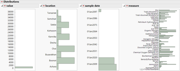
A basic distribution view is generated on the 4 key variables identified for analysis.
Value
This field represents the readings of samples collected. An overwhelming majority (99.5%) fall under 347 and below, while the maximum is at 37959.28. While it is noted that the values are represented on different scales according to the 'Unit' variable, normalisation is not recommended to rescale these values as chemicals naturally occur at widely different levels of amount in soil.
Taking the largest unit of mg/l and maximum value of 37959.28, the value translates to roughly 37.9grams per litre; this indicates the absence of abnormal or impossibly high data errors.
Location
From the table below, we see a wide disparity between the total number of readings collected at each location. This is disconcerting as it indicates a lack of consistency in collection of the chemical samples.
| Location | No. of records |
|---|---|
| Achara | 2855 |
| Boonsri | 31314 |
| Busarakhan | 7492 |
| Chai | 31245 |
| Decha | 2731 |
| Kannika | 22152 |
| Kohsoom | 7895 |
| Sakda | 21429 |
| Somchair | 7537 |
| Tansanee | 2174 |
Dates
The dates do not reflect normally in JMP, whereby the year appears to be inflated. However, no further cleaning was performed on this field as it suitably reads and displays accurately in Tableau.
Measure
The distribution of measures show an even more astonishing disparity in readings between chemicals than the locations. As the data set does clearly show a sizeable amount of zero-value readings (9700), we cannot safely assume that the lack of readings for any particular chemical is due to it not being found in the soil samples.
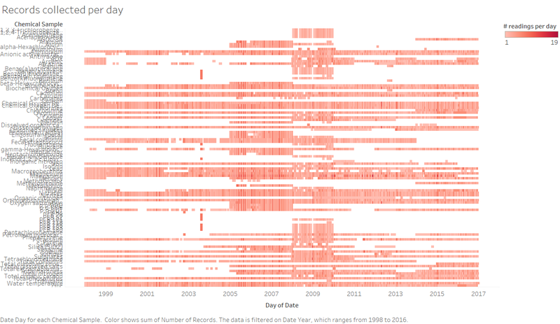
Using a simple colour chart below, a daily view of the collected readings can be shown - at one glance, the records collected for each chemical on a daily basis is highly inconsistent, mostly hovering at just 1, and going as high as 19. This demonstrates a fatal flaw in the collection of the data from a statistical standpoint - insufficient resampling to support any significant observation or hypothesis. It is also not in line with common soil sample collection methodologies.
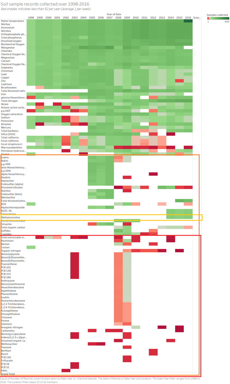
While a daily regimen of sample collection may be too rigid and difficult, another perspective would be to consider an average of 1 collection per week . However, such a view (see chart below) reveals a large number of chemicals having less than this suggested 1 per week average, with a significantly huge number of gaps in collection altogether; these are highlighted in orange.
It is also important to note that the chemical in question, Methylosmoline, also falls under the bucket of chemicals that suffer from these data deficiencies. The only redeeming factor is that it still has 3 years worth of data to review from 2014 to 2016.
For nearly half the chemicals, the data deficiency is so serious that they can be considered to be discarded as they are meaningless for analysis (outlined in red).
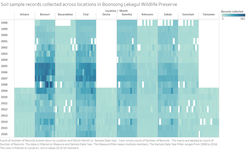
In addition, we can illustrate the number of records collected across all 10 locations and 19 years. From the chart below, it is clear that there were no records collected at 3 locations Achara, Decha, Tansanee for the years 1998-2008. We further note that Boonsri and Chai have an unproportionately larger number of records collected from 2005-2008. Given these observations, it would be most appropriate to take 2009-2016 data for comparisons.
Data Transformation
Given the preliminary observations and exploration conducted above, the visual analysis would be centred on the presentation of the chemical readings against other variables such as location and time.
As noted earlier, the chemical readings are based in varying measurement units. However, it may not be recommended or even be appropriate to normalise them onto the same numerical scale considering the range of values, as well as the fact that naturally occurring readings simply have differing scales in quantity. In addition, as one of the chemicals (Macrozoobenthos) is not listed with any type of measurement, it would be a challenge to transform its readings.
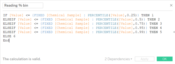
To overcome potential challenges in visually differentiating or comparing between chemicals, bins based on the percentiles can be used. This is done in Tableau by creating a new calculated field using the following code:
The code takes the existing value and considers its percentile value within all readings of the same chemical across every location, then assigns it to a bin from 1 to 6. The percentile values of all locations are considered to better demonstrate significant differences in readings between locations. The bin thresholds have been arbitrarily set to help segregate extreme values which exceed 90% and 95% percentiles. These extreme bins will then be helpful to visually spot extreme values, even when comparing across chemicals, locations and time frames.
Tools
The following tools were used for this exercise:
- Microsoft Excel
- JMP Pro 13.1.0
- Tableau Desktop
