Maptimization Details
Contents
Motivation and Problem Discovery
Motivation
With families in Singapore moving towards modern times where both parents or couple work full-time, domestic household chores are performed much less due to time-constraints. Jelivery Service(JS) Pte Ltd aims to alleviate this issue by providing convenient laundry washing services.
Problem
Currently, Jelivery Services operations function on delivering laundry to each customer's doorsteps regardless of distribution demand nor distance. This creates an issue where deliveries are sometimes time-inefficient and very fuel-consuming for its employees. This results a high operational cost on the company's expenses, making their profit margin very thin.
Proposed Solution
Our group, Maptimization, aims to optimize Jelivery Service's business process by streamlining it via the creation of single-best-point(s) for laundry collections/returns based on the layout of the area and zone. This would increase efficiency and ultimately improve customer satisfaction by providing the best convenience to them possible. Through the use of K-means clustering and sufficient data points, we would be able to create an optimization model.
Solution and Implementation
Approaches
Elbow method
Kmean clustering is to define clusters such that the total intra-cluster variation [or total within-cluster sum of square (WSS)] is minimized. The total WSS measures the compactness of the clustering and we want it to be as small as possible. The Elbow method looks at the total WSS as a function of the number of clusters: One should choose a number of clusters so that adding another cluster doesn’t improve much better the total WSS.
The optimal number of cluster take on the following steps: 1. Compute clustering algorithm (e.g., k-means clustering) for different values of k. For instance, by varying k from 1 to 10 clusters. 2. For each k, calculate the total within-cluster sum of square (wss). 3. Plot the curve of wss according to the number of clusters k. 4. The location of a bend (knee) in the plot is generally considered as an indicator of the appropriate number of clusters.
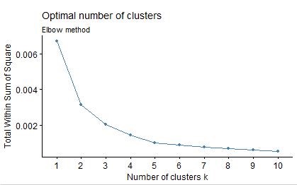

From the above result, we observe that the decrease in marginal different start to occur around k=5, which recommend the optimal number of k cluster to be 5.
Average silhouette method
Average silhouette method The average silhouette approach we’ll be described comprehensively in the chapter cluster validation statistics (Chapter @ref(cluster-validation-statistics)). Briefly, it measures the quality of a clustering. That is, it determines how well each object lies within its cluster. A high average silhouette width indicates a good clustering. Average silhouette method computes the average silhouette of observations for different values of k. The optimal number of clusters k is the one that maximize the average silhouette over a range of possible values for k (Kaufman and Rousseeuw 1990). The algorithm is similar to elbow method which take on the following steps: 1. Compute clustering algorithm (e.g., k-means clustering) for different values of k. For instance, by varying k from 1 to 10 clusters. 2. For each k, calculate the average silhouette of observations (avg.sil). 3. Plot the curve of avg.sil according to the number of clusters k. 4. The location of the maximum is considered as the appropriate number of clusters.
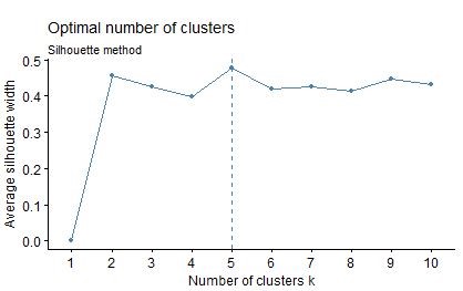

From the above result, we observe that the decrease in marginal different start to occur around k=5, which then recommends the optimal number of k cluster to be 5 to the user.
Gap statistic method
The gap statistic has been published by R. Tibshirani, G. Walther, and T. Hastie (Standford University, 2001). The approach can be applied to any clustering method. The gap statistic compares the total within intra-cluster variation for different values of k with their expected values under null reference distribution of the data. The estimate of the optimal clusters will be value that maximize the gap statistic (i.e, that yields the largest gap statistic). This means that the clustering structure is far away from the random uniform distribution of points. The algorithm works as follow:
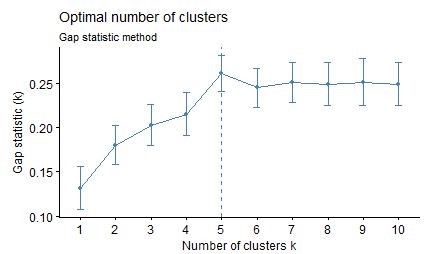

The above result shows that the optimal number of k is 5.
Conclusion: Through the utilization of three analysis's methods, we have found the optimal number of k-cluster to be 5.
Project Sketch
First sketch

Our first sketch sets a direction of what we would like users to be able to see and utilize in our final application. As seen above, we would like to provide three features to our users
1. Filtering by Region(North, South, East, West): This would allow users of different regions to only select laundry collection points near their regions. This is to facilitate convenience and disallow "noise(undesired)" collection points from showing up in their interface
2. Filter by Distance: This means that each collection point can only go up to a certain range from them(e.g. 1KM away from them). The application would recommend how many collection points are within the selected range
3. Filter by K-Clusters: This would allow users to know how many collection points are clustering together, as each collection point is catered to 10 household collection point. If a cluster is more dense, he will more likely be able to collect his laundry easier.
Final sketch

Our final sketch shows an in-depth view of what we would expect the application to look and feel like. Through the selection of options on the top right of our application, users will be able to select Jelivery Service laundry collection points to their own convenience.
For illustration purposes, we have shown that a user have selected the "North" Region and a K-Cluster of 3. The application shows that 3 K-Clusters are shown to the user. The user will then be able to make their way down to whichever is the nearest collection point or whichever is the densest cluster to be served quicker.
Technologies used
Technologies:
- R Shiny
- R Studio
- R Language
- OMS
- Excel
Challenges & Limitations
Data
- There was lack of sufficient data available for Toa Payoh
- Datasets found are often incomplete or had missing fields
Data cleaning and transformation
- Addresses found often had invalid postal codes or unknown postal codes, which required research to amend it
- Data transformation to respective regions(North/South/East/West) was resource-draining and tedious
Novel technologies
- Steep learning curve
- A lot of consultations were needed with Prof Kam
- Self-learning
Future work
This Spatial Clustering with kmean is an optimization model in aiding business to analyze the best collection point or clustering for business needs.
With the option to upload own data set, it would allow the flexibility to be transferable to other business functions and industry as long as they met the data set requirements.
Furthermore, base on the needs of the business, this model can be easily extended to include criteria in its consideration when doing spatial clustering.
For example, we can add in distance into consideration such that the minimum number of distance should not be under 10km or maximum distance should not be over 15km. These would ensure a more fair distribution of k clustering base on the business needs.