Group 8 Application
|
|
|
|
|
Application Web Address
The application has been uploaded onto the following URL for your usage/viewing:
https://timeseriesexplorer.shinyapps.io/timeseriesexplorer/
User Guide
Please refer to the below steps for how to use the system.
Step 1:
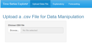
When the app loads, users can click on the "Browse..." button in the "Upload Data File" tab, to select a time-series data .csv file to upload.
Step 2:
After the upload is complete, users can see several sections of information.
On the left-hand side panel, the table displays the various column names (Name), data type (Type), the count of missing records (Mis Value), as well as the position of the missing values (First Mis Value, Last Mis Value).
The main screen on the right, will show a preview of the uploaded data, complete with filter, search, paging and sorting functions.
Step 2.1 (optional):
- If the uploaded dataset does not have a datetime column for time-series analysis, users have an option to click on "Add Index", to generate a new column named "newIndex" that is essentially a running number index column. This will then be converted into a pseudo-datetime column for visualization later.
- Users can also click on the "Transpose The Uploaded Dataset" radio button to perform some data transformations from row to column. After selecting the "From:" and "To" field, enter in the newly renamed "Column Name of Category" and "Column Name of Accumulated Value", before clicking on the "Resume/Transpose Data" button. The transposed columns will appear at the far-right of the preview table.
- For any desire to revert any changes made, simply click on the "Resume to The Original Dataset" radio button, and click again on the "Resume/Transpose Data" button to revert all changes back to the original dataset.
- Users can also click on the "Download" button to download the transformed dataset onto their local drive.
Step 3:
Click on the "Explanatory" tab, and there are many filter options to use at the left-hand panel. In the "Select Column:" section, choose the data columns for "Time-Series Value", "Time Index" and "Category" to dynamically load the type of attributes to filter.
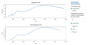
The main screen will display the time-series chart for the main observation data selected, along with its decomposed Seasonal, Trend and Random components.
These charts are useful to understand the behaviour of the time-series data.
Users can then change the "Categorical Attribute", "Date start with no missing value" and "Period" fields to filter out the records.
For the "Customise Visualisation" section, there is also an option to denote whether the time-series data is "multiplicative" or "additive".
Seasoned analysts would know that the calculations done for these two types of time-series data are quite different.
The "Time Series Frequency" can also be set, with the default value of "12" to denote months in a year.
Step 3.1 (optional):
Users can also filter out the sub-graphs by clicking on their respective checkboxes at the end.
Step 4:
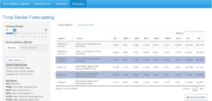
After making the selections from the left-hand panel, click on the "Forecasting" tab to allow the system to run a series of calculations to find the best parameters for both Exponential Smoothing and ARIMA models.
After giving it sometime, a table will be generated on the main screen. These are the best models chosen for their lowest AIC/BIC values and users can compare the various accuracy scores (based on train data only).
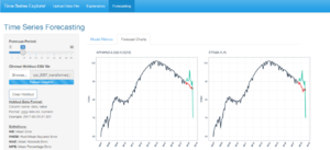
Users can then click on the various rows for closer scrutiny and click on the "Forecast Charts" tab to generate line charts with their respective forecasts.
The "Forecast Period" slider on the left hand panel allows users to select how far ahead the charts can forecast up to.
To save the model parameters, click on the "Download Stats" button. To save the charts, simply right-click and copy the charts to the clipboard or save manually.
Step 4.1 (optional):
There is also an option for the user to upload "Holdout data" by clicking on the browse button under the slider.
Once uploaded, the charts will automatically reflect the additional actual data in the line charts, for comparison with the predicted values.
Click on the "Clear Holdout" button to clear the holdout line from the charts.
Feedback
We appreciate your feedback, please send us any comments via the email addresses below:
guoteng.fam.2016@mitb.smu.edu.sg
yanru.xu.2016@mitb.smu.edu.sg
yuchen.wang.2016@mitb.smu.edu.sg


