ISSS608 2016-17 T3 Assign CHEN XIAOQING

Background

Ornithology student Mitch Vogel was immediately suspicious of the noxious gases just pouring out of the smokestacks from the four manufacturing factories south of the nature preserve. He was almost certain that all of these companies are contributing to the downfall of the poor Rose-crested Blue Pipit bird. But when he talked to company representatives and workers, they all seem to be nice people and actually pretty respectful of the environment.

In fact, Mitch was surprised to learn that the factories had recently taken steps to make their processes more environmentally friendly, even though it raised their cost of production. Mitch discovered that the state government has been monitoring the gaseous effluents from the factories through a set of sensors, distributed around the factories, and set between the smokestacks, the city of Mistford and the nature preserve. The state has given Mitch access to their air sampler data, meteorological data, and locations map. Mitch is very good in Excel, but he knows that there are better tools for data discovery, and he knows that you are very clever at visual analytics and would be able to help perform an analysis.

Mini-Challenge 2 provides a three month set of data for you to analyze, covering April, August, and December 2016.

Objectives/Questions

1. Characterize the sensors’ performance and operation. Are they all working properly at all times? Can you detect any unexpected behaviors of the sensors through analyzing the readings they capture?Limit your response to no more than 9 images and 1000 words.
2. Now turn your attention to the chemicals themselves. Which chemicals are being detected by the sensor group? What patterns of chemical releases do you see, as being reported in the data? Limit your response to no more than 6 images and 500 words.
3. Which factories are responsible for which chemical releases? Carefully describe how you determined this using all the data you have available. For the factories you identified, describe any observed patterns of operation revealed in the data. Limit your response to no more than 8 images and 1000 words.

Data Descriptions

Overview

This data consists of sensor readings from a set of air-sampling sensors and meteorological data from a weather station in proximity to the factories and sensors.

The factories and sensors locations are provided in terms of x,y coordinates on a 200x200 grid, with (0,0) at the lower left hand corner (southwest).

The following are the factory locations:

Roadrunner Fitness Electronics: 89,27

• Kasios Office Furniture: 90,21
• Radiance ColourTek: 109,26
• Indigo Sol Boards: 120,22

The following are the sensor locations:

• 1: 62,21
• 2: 66,35
• 3: 76,41
• 4: 88,45
• 5: 103,43
• 6: 102,22
• 7: 89,3
• 8: 74,7
• 9: 119,42

Companies

Manufacturing Companies near Mistford:

• Roadrunner Fitness Electronics – Roadrunner produces personal fitness trackers, heart rate monitors, headlamps, GPS watches, and other sport-related consumer electronics. Roadrunner began as one of the region’s first fitness stores in 1962, with an eye toward outfitting the entire nation with appropriate outdoor gear. After an earthquake nearly destroyed their main warehouse in 1968, Roadrunner turned a bad situation into a glowing success with the first “slightly damaged goods” sale. After which they began to focus on manufacturing; though their “Earthshaking Bargains” business still sells dented, overstocked and refurbished items over the internet and from a small retail shop attached to their front office.
• Kasios Office Furniture – Kasios Office Furniture manufactures metal and composite-wood office furniture including desks, tables, and chairs. Kasios wants to do with desk chairs what Starbucks did for coffee – making office furniture what people must have, instead of what they just need. “Office equipment doesn’t need to be ugly!” says founder Ken Kasios. “We have redesigned all office products to be cool, fun, and hip—even your basic stapler.” Kasios business model is focused on in-store merchandising highlighting the beauty and functionality of their “user-centered design”. They recently celebrated the one-year anniversary of a distribution and merchandising agreement with the national office supply chain store PaperKlips.
• Radiance ColourTek – Radiance produces solvent based optically variable metallic flake paints. “Metallic paints with an untarnished reputation!” quips ColourTek’s Senior Vice President Arthur Donner. “Radiance ColourTek metallic paints are worth their weight in gold.” Offering a new generation of paints in the 1970s, Radiance out marketed all competitors for three decades until manufacturing process issues began to tarnish their reputation. “We were challenged,” said Donner. “Polishing up our pearlescent pigments caused us to lose luster, but now we have the lowest VOCs (volatile organic compounds) in the industry!”
• Indigo Sol Boards – Indigo Sol produces skateboards and snowboards. Founder Billy Keys started off manufacturing wooden wine barrels for northwestern US wineries, but then navigated a course from decorative fiberglass wine barrels to making his first pair of fiberglass skis in 1971. Excellent product and sales decisions rocketed Keys Skis production to unexpected levels, until they were bought out by a large Denver, Colorado-based private investment group. Keys returned to making specialized snowboards in the 1980s, with a small company in Mistford called Indigo Sol. The company has seen modest growth in recent years.

Chemicals

• Appluimonia – An airborne odor is caused by a substance in the air that you can smell. Odors, or smells, can be either pleasant or unpleasant. In general, most substances that cause odors in the outdoor air are not at levels that can cause serious injury, long-term health effects, or death to humans or animals. However, odors may affect your quality of life and sense of well-being. Several odor-producing substances, including Appluimonia, are monitored under this program.
• Chlorodinine – Corrosives are materials that can attack and chemically destroy exposed body tissues. Corrosives can also damage or even destroy metal. They begin to cause damage as soon as they touch the skin, eyes, respiratory tract, digestive tract, or the metal. They might be hazardous in other ways too, depending on the particular corrosive material. An example is the chemical Chlorodinine. It has been used as a disinfectant and sterilizing agent as well as other uses. It is harmful if inhaled or swallowed.
• Methylosmolene – This is a trade name for a family of volatile organic solvents. After the publication of several studies documenting the toxic side effects of Methylosmolene in vertebrates, the chemical was strictly regulated in the manufacturing sector. Liquid forms of Methylosmolene are required by law to be chemically neutralized before disposal.
• AGOC-3A – New environmental regulations, and consumer demand, have led to the development of low-VOC and zero-VOC solvents. Most manufacturers now use one or more low-VOC substances and Mistford’s plants have wholeheartedly signed on. These new solvents, including AGOC-3A, are less harmful to human and environmental health.

Analytic Results and Answers

Question 1

1-1

To characterize the performance of each monitor, first use the line chart to compare the reading in every time stamp with the overall median reading value, whether the reading in this time stamp is higher or lower than the median value. Then characterize how the monitor performs and operates through the whole period.

The line chart consists of two lines in each monitor panel. One line is the reading of this monitor, another one is the overall median value. It has four chemicals and each chemical detected characteristics is not the same, so it’s not reasonable to sum them up. It does more sense to see the monitors operates with each chemical. The same reason for looking at individual month. So here placed two filters, by month and by chemical. The whole dashboard is like right graph 1-1:

Findings:

Finding 1:

Above graph indicates the reading of four chemicals of each monitor in April. The X-axis is the hour of each day in April, while the Y-axis represents the monitors. Compare the reading of these four pollutions through whole period, the characteristics are shown below:

• Monitor 3, 7 and 8 are consistently detecting the relative higher reading value compare to the median reading of four chemicals.
• The reading detected by rest monitors (1, 2, 4, 5, 6 and 9) along this month is consistently fluctuated around the median reading value with some cases that detect relative higher value above the median value in all chemicals. (monitor 1 and 2 have very few cases that detect relative higher values.)
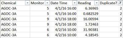
• Note that the number of cases of detecting relative higher value is much higher in detecting AGOC-3A than detecting others. The reason probably is the duplicated records of reading this chemical. (there are 168 records with same time stamp, same monitor but two different reading records) Another reason may be this kind of chemical is more actively released in this park.

Finding 2:

The characteristics of monitors in August are slightly different with those in April.

• Not only monitor 3 and 7 but also monitor 4 are consistently detect values higher than median.
• Monitor 1, 2, 8 and 9 detect the values just around the median with very few cases that will much higher than the median. While the rest monitors have read more cases with higher value.

Finding 3:

• Monitor 3, 4, 5, 7 and 9 always have read the relative higher value than median during this month. The reading of 9 is just slightly higher than the median.
• Monitor 1, 2, 6 and 8’s readings fluctuated around the median value. Only the monitor 6 in detecting AGOC-3A has higher variance.

Conclusion:

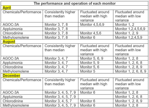
From the conclusion table we can see the monitors have three main performances in reading the chemicals. There are two main finding in the performance of all the monitors:

• The monitor 3 has always read the consistent higher value in all moths and all chemicals.
• Monitor 1 and 2 have caught the fluctuated reading around median all the time no matter what the chemicals and whenever the months.

These two behaviors may be considered as unexpected performances due to consistent the same behavior. We have higher possibility to suspect that they may not be working properly all the time because the performance of both monitor 3 and 1&2 has remained the same all the time no matter what the chemical is and which moth it is in. What’s more, the reading detected by sensor 3 is much higher than the median at all situations.

Take a closer look at the unexcepted behaviors using the horizon graph. The horizon graph of all the reading through three months shows the difference between individual reading and median value in a same horizon, using orange-green diverging color to represent the positive and negative value. The density of color represents the level of difference from median. The darker the color is, the higher it differs from median.

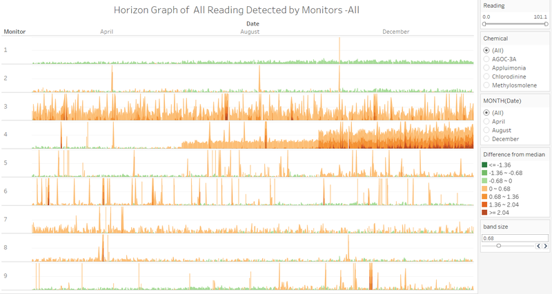
First take a look at the monitor 1, which represents as consistently slight lower than the median through this whole period. As previous analysis showed, the reading of monitor 1 fluctuated around median, which here obviously is wrong. The reason probably is the reading of monitor 1 is very slightly lower than the median and we cannot see it clearly at first look. Although it’s different from previous result, the monitor 1 still may be not working properly all the time. The performance always tends to read lower value consistently.

Then is the monitor 2, both the green and orange have taken up almost half percentage with relative low variance. This is identical to previous analysis. The level of difference between reading of monitor 3 and median is very high during all the time. Many time stamps have reached the highest level.

Interestingly, monitor 4 also seems not to be working properly all the time. It performs differently during all three months, which represents around median, relative higher than median and much higher than median in April, August and December respectively.

Question 2

1) To determine which chemicals are mainly be detecting by sensor group, we’d better use the boxplot to see the reading distribution of each chemical in each monitor. Define the top-3 covered quartile size into the main sensor group.

Below table shows the conclusion of grouping sensors for detecting each chemical through the distribution of reading in three months.

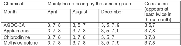
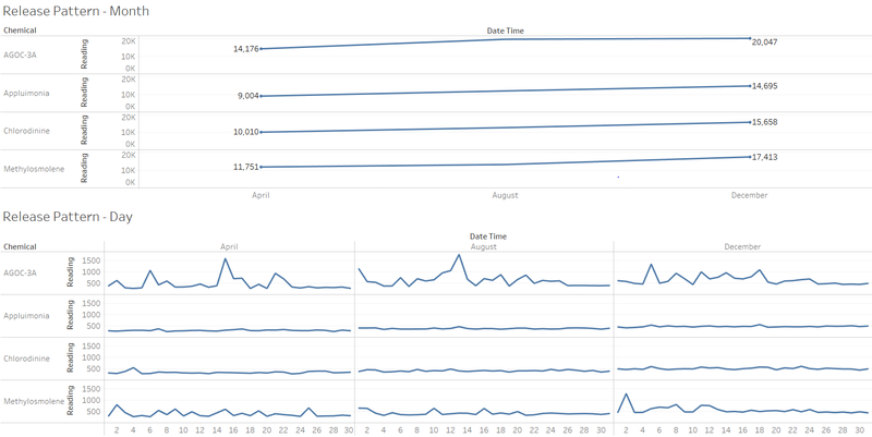
2) Chemical Release Pattern:

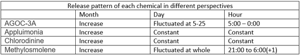
• Looking the reading month by month, it shows the total release of each chemical has an upward trend from April to December. Then looking it day by day in each month, the release of Appluimonia and Chlorodinie remains almost the same in the whole month (not changing too much), which the AGOC-3A and Methylosmolene have their specific pattern. The release patterns of AGOC-3A in three months are quite similar, which has been fluctuating during around 5-25 days. The release pattern of Methylosmolene remained consistent during the most days in whole month but there are some irrgular days fluctuated a lot.

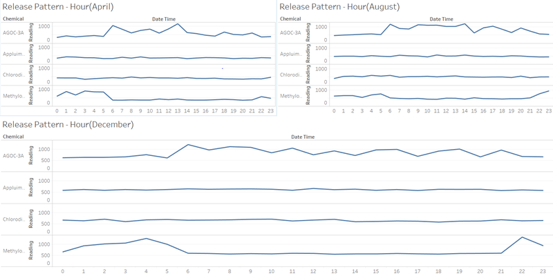
• Below gragh is to see the release pattern in persepctive of hour in a day. It’s obivious that the release pattern of Appluimonia and Chlorodinie remains constant through whole day. But the AGOC-3A release is mainly gathered from 5:00 – 0:00, while Methylosmolene is mainly collected from 21:00 to 6:00 in the next day.

Conclusion: