Difference between revisions of "The Indian Story Data Prep"
| (One intermediate revision by the same user not shown) | |||
| Line 77: | Line 77: | ||
<pre> | <pre> | ||
| + | library(tidyverse) | ||
| + | |||
table1<- readxl::read_excel("Table 1.xlsx") | table1<- readxl::read_excel("Table 1.xlsx") | ||
table2 <- readxl::read_excel("Table_2_PR_Cities_1Lakh_and_Above.xls", skip = 5, col_names = F) | table2 <- readxl::read_excel("Table_2_PR_Cities_1Lakh_and_Above.xls", skip = 5, col_names = F) | ||
| Line 153: | Line 155: | ||
===Solution === | ===Solution === | ||
| − | The solution involved replacing the missing words with the corresponding correct codes | + | The solution involved replacing the missing words with the corresponding correct codes. |
<pre> | <pre> | ||
| − | gather_table$Literacy_Standard[gather_table$Literacy_Standard == "BelowPrim"] <- c("BelowPrimary") | + | gather_table$Literacy_Standard[gather_table$Literacy_Standard == "BelowPrim"] <- c("Below Primary") |
| + | gather_table$Literacy_Standard[gather_table$Literacy_Standard == "BelowPrimary"] <- c("Below Primary") | ||
gather_table$Literacy_Standard[gather_table$Literacy_Standard == "illiterate"] <- c("Illiterate") | gather_table$Literacy_Standard[gather_table$Literacy_Standard == "illiterate"] <- c("Illiterate") | ||
gather_table$Literacy_Standard[gather_table$Literacy_Standard == "L_NoEdu"] <- c("Literate (No-Education)") | gather_table$Literacy_Standard[gather_table$Literacy_Standard == "L_NoEdu"] <- c("Literate (No-Education)") | ||
| − | + | gather_table$Literacy_Standard[gather_table$Literacy_Standard == "S"] <- c("Secondary") | |
| − | + | gather_table$Literacy_Standard[gather_table$Literacy_Standard == "M"] <- c("Middle School") | |
| − | + | gather_table$Literacy_Standard[gather_table$Literacy_Standard == "P"] <- c("Primary") | |
| − | + | gather_table$Literacy_Standard[gather_table$Literacy_Standard == "PreUni"] <- c("Pre-University") | |
| + | gather_table$Literacy_Standard[gather_table$Literacy_Standard == "Diploma_NT"] <- c("Diploma (Non-Technical)") | ||
| + | gather_table$Literacy_Standard[gather_table$Literacy_Standard == "Diploma_T"] <- c("Diploma(Technical)") | ||
</pre> | </pre> | ||
| + | The output is as shown in the summary as bellow. <br/> | ||
| + | [[File:Summary df.JPG|1000px]] | ||
Latest revision as of 18:58, 22 July 2017
Contents
- 1 Data
- 1.1 Data as downloaded from the website
- 1.2 Data Problem 1: Break the hierarchy
- 1.3 Data Problem 2: State Codes are not Sufficient!
- 1.4 Data Problem 3: The Table has too many variables and is too broad
- 1.5 Data Problem 4: "Literacy Level" is still not purely Literacy level"
- 1.6 Data Problem 5: The "Town Name" was not pure enough
- 1.7 Data Problem 6: Categories unclear under "Literacy Standard" variable
Data
Here we speak about the dataset and munging that we do upon it. In order to create the visualisations and eventually build the Application it is important to have the data in the right form. Let's start with examining the data in its initial form.
Data as downloaded from the website
The copy of the data can be downloaded from this link here
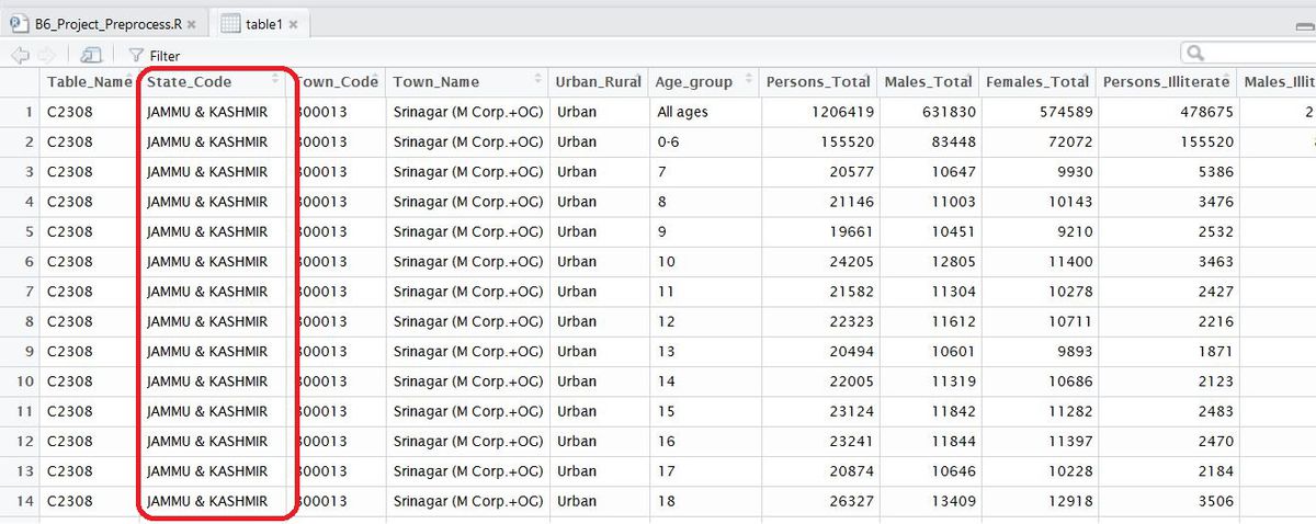
Here is a portion of the data excel data source that somewhat gives us an overview of the data. I'll explain more in the tables below. Sometimes visually looking at the data helps flare off ideas on how to munge it.
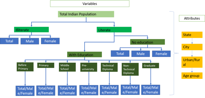
The data file is quite a clean file with no missing values. Those with no values are replaced with 0 and they are all in terms of population numbers. No ratios have been computed except for totals. A glance at the data file above will give you the impression that there is more than one level of data and that information is in the hierarchical form. The picture below is what we visualise the dataset to be conceptually.
Every row has certain data attributes. Population information in each row has a hierarchial structure beginning with the state code followed by the city/town name then whether it is an Urban or a rural city and finally the age group. Here however there isn't a particular state name given for the state code. This is where the second dataset comes in and helps us understand the meaning of the state codes.
Next the variables also have a hierarchial structure. You have the highest level popluation totals. These tell you total population, total male population and total female population. Then following that you have the division of Illiterate and Literate population numbers. Both of these have persons, male and female divisions. Next under Literate you have those with education and those without education. Again under Literate and without education you have population total number of male and female numbers. Then under Literate with education, you have the different levels of education! They go all the way from before Primary to Graduates. Then under each of these categories you have population numbers for total, male and female.
So let's start addressing one data problem after another. The following explains the problem and the solution used to solve them.
Data Problem 1: Break the hierarchy
Problem
So the dataset itself came with a hierarchy which needed to be broken down.
Solution
This was done in R. We assign the new column names to the data frame as below. This dataset was then stored as "Table 1.xlsx".
library(openxlsx)

DDWCT <- read.xlsx("DDWCT-0000C-08.xlsx", sheet = 1, startRow = 8, colNames = F)

new_col_names <- c("Table_Name", "State_Code", "Town_Code", "Town_Name", "Urban_Rural", "Age_group", "Persons_Total", "Males_Total", "Females_Total", "Persons_Illiterate",
                                  "Males_Illiterate", "Females_illiterate", "Persons_Literate", "Males_Literate", "Females_Literate", "Persons_L_NoEdu", "Males_L_NoEdu", "Females_L_NoEdu",
                                  "Persons_BelowPrim", "Males_BelowPrim", "Females_BelowPrimary", "Persons_P", "Males_P", "Females_P", "Persons_M", "Males_M", "Females_M", "Persons_S",
                                  "Males_S", "Females_S", "Persons_PreUni", "Males_PreUni", "Females_PreUni", "Persons_Diploma_NT", "Males_Diploma_NT", "Females_Diploma_NT",
                                  "Persons_Diploma_T", "Males_Diploma_T", "Females_Diploma_T", "Persons_Graduates", "Males_Graduates", "Females_Graduates", "Persons_Unclassified",
                                  "Males_Unclassified", "Females_Unclassified")

names(DDWCT) <- new_col_names

write.xlsx(DDWCT, file = "Table 1.xlsx", colNames = T)
Data Problem 2: State Codes are not Sufficient!
Problem Definition
Imagine if you read a map, hover over a particular state in India and all you get to see is the state code. Unless you are an educated Indian, you wouldn't know what that means. Hence the second dataset was used. This can be downloaded here
Solution
We wrote a beautiful R code to munge this.
library(tidyverse)

table1<- readxl::read_excel("Table 1.xlsx")
table2 <- readxl::read_excel("Table_2_PR_Cities_1Lakh_and_Above.xls", skip = 5, col_names = F)

cl_table2 <- table2[, 1:2] %>% distinct()

for(i in 1:nrow(cl_table2)) {
  state_row <- cl_table2[i, ]
  table1$State_Code[table1$State_Code == state_row[[1]]] <- state_row[[2]]
}
Data Problem 3: The Table has too many variables and is too broad
Problem
Data lessons say that it is easier to work with data tables that are narrow. This table was too broad with many variables. These variables could be converted to categories instead and put into a column.
Solution
We used the gather function of the tidyverse library in R
library(tidyverse)

#Gather table
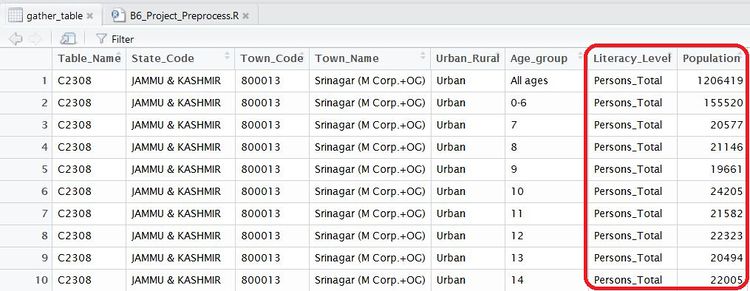
gather_table <- table1 %>% gather("Literacy_Level","Population", 7:45)
The output of the following code looked like this :
The columns now are broken down to one categorical variable called "Literacy Level" and a numerical variable "Population"
Data Problem 4: "Literacy Level" is still not purely Literacy level"
Problem
The issue now is the with the "Literacy Level" column. A quick examination of the screenshot above will show that it also includes information of Persons, Male and Female. This information is delimited from the actual literacy level information by a "_" character.
Solution
This could be easily solved with the separate function in the package tidyr.
library(tidyr)

gather_table <- separate(gather_table, Literacy_Level, into = c("Type_Level", "Literacy_Standard"), sep = "_", extra = "merge")
Now the table is look like as below.
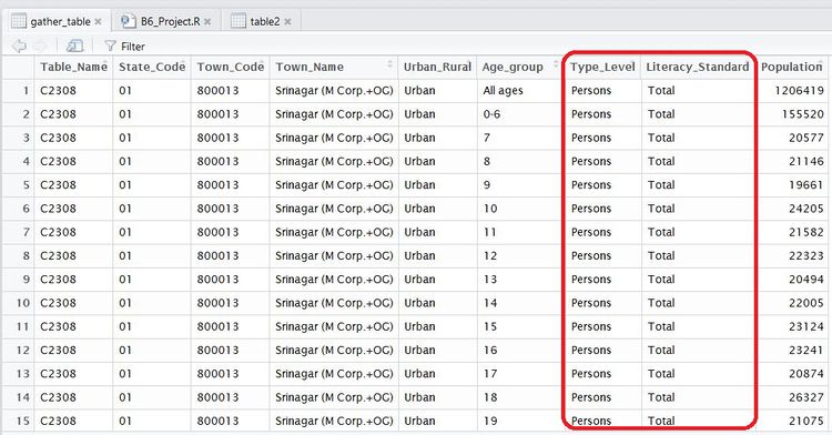
Data Problem 5: The "Town Name" was not pure enough
Problem
This was a similar problem as above. Town Names were accompanied with additional information such as (M Corp. + OG) as seen above in Srinagar (M Corp.+ OG).
Solution
The same separate function was used to separate the this column and extract only the town names. "(" character was used as a delimiter and the column containing (M Corp. + OG) values was deleted.
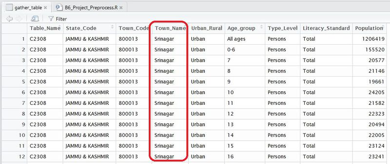
gather_table <- separate(gather_table, Town_Name, into = c("Town_Name"), sep = " \\(", extra = "drop")
The resultant table looked like this:
There is another column called "Type level" that contains information about Persons, Male or Female and the "Town Name" contains only the town name.
Data Problem 6: Categories unclear under "Literacy Standard" variable
Problem
Here is an R summary of the data file shown above. It particularly shows the categories present in the "Literacy Standard" variable. This wasn't clean enough as there are two Below Primary values. There are two "illiterate" categories. There is also a "L_NoEdu" column. This issue arose from the manual merging of the table in the very first step. Refer to Data Problem 1.
> summary(as.factor(gather_table$Literacy_Standard))
   BelowPrim   BelowPrimary   Diploma_NT    Diploma_T    Graduates   illiterate   Illiterate      L_NoEdu     Literate            M            P       PreUni            S       Total   Unclassified
          29290               14645             43935            43935          43935       14645      29290          43935        43935     43935     43935       43935    43935     43935             43935
Solution
The solution involved replacing the missing words with the corresponding correct codes.
gather_table$Literacy_Standard[gather_table$Literacy_Standard == "BelowPrim"] <- c("Below Primary")
gather_table$Literacy_Standard[gather_table$Literacy_Standard == "BelowPrimary"] <- c("Below Primary")
gather_table$Literacy_Standard[gather_table$Literacy_Standard == "illiterate"] <- c("Illiterate")
gather_table$Literacy_Standard[gather_table$Literacy_Standard == "L_NoEdu"] <- c("Literate (No-Education)")
gather_table$Literacy_Standard[gather_table$Literacy_Standard == "S"] <- c("Secondary")
gather_table$Literacy_Standard[gather_table$Literacy_Standard == "M"] <- c("Middle School")
gather_table$Literacy_Standard[gather_table$Literacy_Standard == "P"] <- c("Primary")
gather_table$Literacy_Standard[gather_table$Literacy_Standard == "PreUni"] <- c("Pre-University")
gather_table$Literacy_Standard[gather_table$Literacy_Standard == "Diploma_NT"] <- c("Diploma (Non-Technical)")
gather_table$Literacy_Standard[gather_table$Literacy_Standard == "Diploma_T"] <- c("Diploma(Technical)")


