IS428 2016-17 Term1 Assign3 Jonathan Eduard Chua Lim
Contents
Questions
As an expert in visual analytics, you have been hired to help GAStech understand its operations data. In this assignment, you are given two weeks of building and prox sensor data. Can you use visual analytics to identify typical patterns of and issues of concern?
You will be asked to answer the following types of questions:
- What are the typical patterns in the prox card data? What does a typical day look like for GAStech employees?
- Describe up to ten of the most interesting patterns that appear in the building data. Describe what is notable about the pattern and explain its possible significance.
- Describe up to ten notable anomalies or unusual events you see in the data. Prioritize those issues that are most likely to represent a danger or a serious issue for building operations.
- Describe up to five observed relationships between the proximity card data and building data elements. If you find a causal relationship (for example, a building event or condition leading to personnel behavior changes or personnel activity leading to building operations changes), describe your discovered cause and effect, the evidence you found to support it, and your level of confidence in your assessment of the relationship.
HVAC Information and its Significance
| Field | Units | Description |
|---|---|---|
| F_#_BATH_EXHAUST:Fan Power | [W] | Power used by the bathroom exhaust fan |
| F_#_VAV_SYS AIR LOOP INLET Mass Flow Rate | [kg/s] | Total flow rate of air returning to the HVAC system from all zones it serves |
| F_#_VAV_SYS AIR LOOP INLET Temperature | [C] | Mixed temperature of air returning to the HVAC system from all zones it serves |
| F_# VAV Availability Manager Night Cycle Control Status | On/off status of the HVAC system during periods when the system is normally scheduled off. The night cycle manager cycles the HVAC system to maintain night and weekend set point temperatures. | |
| F_#_VAV_SYS COOLING COIL Power | [W] | Power used by the HVAC system cooling coil |
| F_#_VAV_SYS HEATING COIL Power | [W] | Power used by the HVAC system heating coil |
| F_#_VAV_SYS SUPPLY FAN OUTLET Mass Flow Rate | [kg/s] | Total flow rate of air delivered by the HVAC system fan to the zones it serves |
| F_#_VAV_SYS SUPPLY FAN OUTLET Temperature | [C] | Temperature of the air exiting the HVAC system fan |
| F_#_VAV_SYS SUPPLY FAN:Fan Power | [W] | Power used by the HVAC system fan |
| F_#_VAV_SYS Outdoor Air Flow Fraction | Percentage of total air delivered by the HVAC system that is from the outside | |
| F_#_VAV_SYS Outdoor Air Mass Flow Rate | [kg/s] | Flow rate of outside air entering the HVAC system |
| COOL Schedule Value | Example | The supply air temperature set point. Air exiting the HVAC system fan is maintained at this temperature during cooling operation |
| DELI-FAN Power | [W] | Power used by the deli exhaust fan |
| Drybulb Temperature | [C] | Drybulb temperature of the outside air |
| Wind Direction | [deg] | Direction of wind outside of the building |
| Wind Speed | [m/s] | Speed of wind outside of the building |
| HEAT Schedule Value | The supply air temperature set point. Air exiting the HVAC system fan is maintained at this temperature during heating
operation | |
| Pump Power | [W] | Power used by the hot water system pump |
| Water Heater Setpoint | Water heater set point temperature | |
| Water Heater Gas Rate | [W] | Rate at which the water heater burns natural gas |
| Water Heater Tank Temperature | [C] | Temperature of the water inside the hot water heater |
| Loop Temp Schedule | Example | Temperature set point of the hot water loop. This is the temperature at which hot water is delivered to hot water
appliances and fixtures. |
| Supply Side Inlet Mass Flow Rate | [kg/s] | Flow rate of water entering the hot water heater |
| Supply Side Inlet Temperature | [C] | Temperature of the water entering the hot water heater |
| Supply Side Outlet Temperature | [C] | Temperature of the water exiting the hot water heater |
| F_#_Z_# REHEAT COIL Power | [W] | Power used by the zone air supply box reheat coil |
| F_#_Z_# RETURN OUTLET CO2 Concentration | [ppm] | Concentration of C02 measured at the zone's return air grille |
| F_#_Z_# SUPPLY INLET Mass Flow Rate | [kg/s] | Flow rate of the air entering the zone from its air supply |
| F_#_Z_# SUPPLY INLET Temperature | [C] | Temperature of the air entering the zone from its air supply |
| F_#_Z_# VAV REHEAT Damper Position | Position of the zone's air supply box damper. 1 corresponds to fully open, 0 corresponds to fully closed | |
| F_#_Z_#: Equipment Power | [W] | [W] Power used by the electric equipment in the zone |
| F_#_Z_#: Lights Power | [W] | Power used by the lights in the zone |
| F_#_Z_#: Mechanical Ventilation Mass Flow Rate | [kg/s] | Ventilation rate of the zone exhaust fan |
| F_#_Z_#: Thermostat Temp | [C] | Temperature of the air inside the zone |
| F_#_Z_#: Thermostat Cooling Setpoint | [C] | Cooling set point schedule for the zone |
| F_#_Z_#: Thermostat Heating Setpoint | [C] | Heating set point schedule for the zone |
| Total Electric Demand Power | [W] | Total power used by the building |
| HVAC Electric Demand Power | [W] | Total power used by the building's HVAC system including coils, fans and pumps. |
Data Preparation
Modifying Employee Information
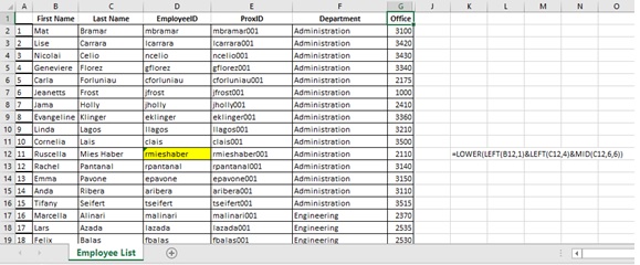
- I created an EmployeeID column using the first letter of the employee’s name and the Full last name.
- Generated Prox ID by using the EmployeeID and adding “001”, denoting their first Prox ID card.
- From looking at Mobile Prox Data (Rosie), I have found that employees with 2 last names (ie. Ada Campo-Corrente) or special characters after their last name (ie. Sten Sanjorge Jr) was transformed to “acampo” and “jsanjorge” respectively.
- The formula and the transformation for these special types of proxid can be seen below.
| First Name | Last Name | Transformed Employee ID | Formula |
|---|---|---|---|
| Ruscella | Mies Haber | rmieshaber | =LOWER(LEFT(B12,1)&LEFT(C12,4)&MID(C12,6,6)) |
| Ada | Campo-Corrente | acampo | =LOWER(LEFT(B53,1)&LEFT(C53,5)) |
| Sten | Sanjorge Jr. | jsanjorge | =LOWER(MID(C58,10,1)&MID(C58,1,8)) |
| Willem | Vasco-Pais | wvasco | =LOWER(LEFT(B60,1)&LEFT(C60,5)) |
Creating Custom Polygon for Tableau
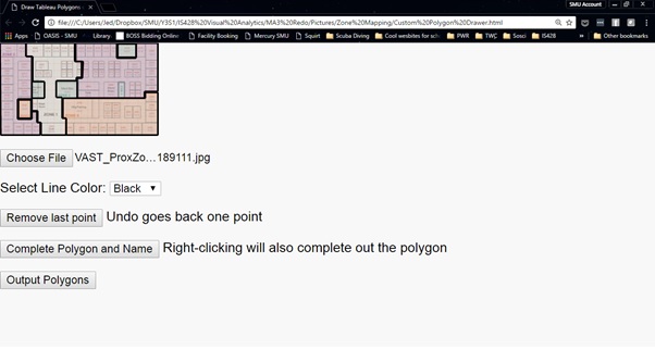
I plotted the Custom Polygon using this tool: [Blog Link] [Github Link]. This tool allowed me to create polygons by allowing you to draw in them, and the exported result is a 4 column: Identifier, Path ID, X and Y Coordinates. These can be used for Tableau to read the polygons and also to calculate the Fixed Prox Data's X and Y coordinates.
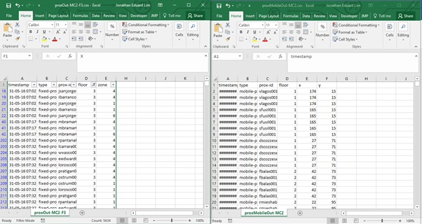
Mobile Prox and Fixed Prox Data:
I found out that the Fixed Prox Data did not have X and Y axis, and that the Mobile Prox Data did not have a zone value allocated to its dataset. The following is my attempt to bridge the gap.
Fixed Prox Data:
My main assumption is that the the Fixed Proximity Sensor is located in one specific part of the respective zone.
Firstly, I plotted the zones in a custom polygon html (Link here) and got the X and Y axis in a separate excel file.
I then used V lookup to generate the X and Y axis for the Fixed Prox Data, with the following formula: =VLOOKUP(E2,[Floor1.xlsx]Sheet1!$A$2:$B$34,2,FALSE) (credit to [James Chua]). Then I was able to generate the X and Y axis for the Fixed Proximity Data.
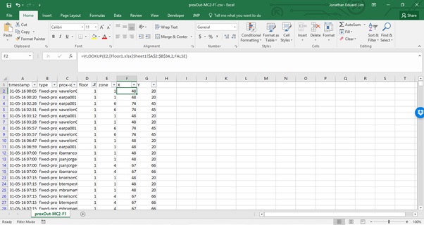
I repeated these steps for Floor # 2 and # 3 respectively. To simplify the analysis, I decided to combine the 2 Proximity Data together in one csv file.
Hazium Concentration
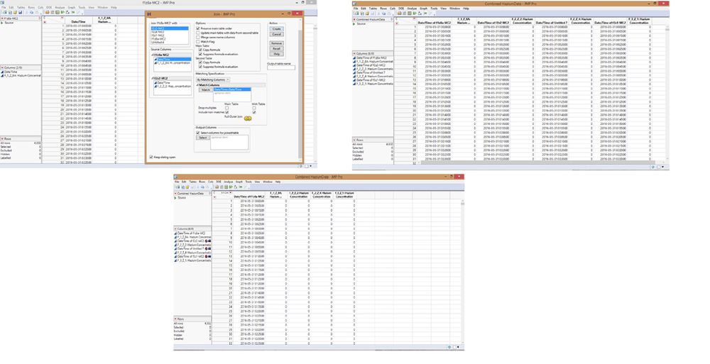
Combined the 4 tables of Hazium Concentration with the following settings. Afterwards, I deleted the common Date/Time column, only leaving 1 date/time column. I joined it using JMP Pro's Join function. I ticked the "include non-mathches" for both Main and With Table column, and did these for each of the tables to combine it into one table.
Preparing HVAC Data
I used the “Stack” function in JMP Pro to convert the columns into rows
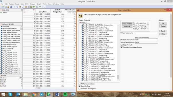
After stacking them, I realized that there are 2 main types of measurement name: those starting “F_#_Z_#” (Floor #,Zone #) and those without. I segregated those without to another file, and joining the two together afterwards.
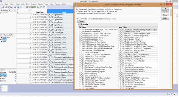
I then used the Standardise Attributes > Recode function under Columns, to ensure that all those measurement names with “F_#_Z_#” are standardized and ready for delimiting. I checked all of them manually to ensure smooth delimiting later on.
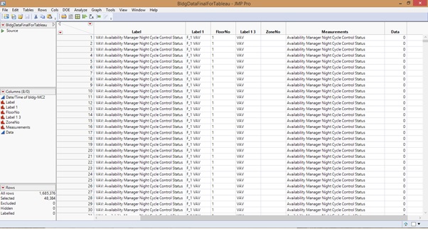
I combined the Hazium Concentration data to the main table. After this, I delimited it by “_” to create a Floor and Zone table. This is so that when the data is uploaded into tableau, it can be filtered by floor and zone. Afterwards I combined the label and data without the starting:“F_#_Z_#”
Findings: Question 1
What are the typical patterns in the prox card data? What does a typical day look like for GAStech employees?
- Rosie starts to deliver letters from 9am and 2pm, going around each floor in an anticlockwise manner, from Floor 1, 2 and 3.
- Most of those in the Executive Department arrive to work around 7am.
- The CEO, Sten Sanjorge, only appear at around 11am. He is also the latest Executive member to leave the office at 6pm.
- The security department patrols each floors of the office regularly throughout the day. They usually patrol at 8am, 12pm, 1pm and 5pm based on their Prox Id count.
- There is no Prox ID count for the Security Department between 11-12 June, which is worrying due to the importance of their job.
- Mat Bramar, an Administration department staff, is only seen in the office on the 11th of June. He is not present at any days other than 11 June.
- The Engineering department are present either in 1st and 2nd floor. They are never seen on the 3rd floor.
- The Facilities team often arrive later than most people, usually at 10am.
- The HR team starts their day at 8am, and end their day at 5pm
- The IT department has the shortest work day amongst the different departments, as short as 2 hours in 7 June 2016. (1 hour in 8 June)
Findings: Question 2
Describe up to ten of the most interesting patterns that appear in the building data. Describe what is notable about the pattern and explain its possible significance
- In Floor 1 Zone 1 (Deli at floor 1), there is a spike of “Lights Power” between 11am-12pm. This signifies lunch time for employees, as most or if not all of the lights are turned on to accommodate for the employees who are having lunch. Also, there is a small increase at 7am, in which could mean that some employees eat breakfast before starting work.
- In Floor 1 Zone 5 (Conference Room), there is a sudden increase of Lights and Equipment power usage between 1am-3am. There seem to be conferences starting from 1am up to 3am. A similar pattern can be seen between 5am-7am, which are another set of conferences.
- Floor 1 Zone 7 (Loading Room with Offices), there are a spike in Equipment Power and Lights Power at these following times: 1am, 4-5am, 7-8am, 3pm-5pm, and 9pm. These could mean that there are either outgoing or incoming deliveries at these time frames.
- Floor 2 Zone 5 (Office number 2300) seem to be used after office hours. This is because there is an increase of Equipment Power and Lights Power used from 3pm to 11pm, with a “break” at 10pm. An employee may be working at these odd hours.
- Floor 2 Zone 16 (Cluster of Offices near Floor 2 Zone 5) seems to be used from 3pm-11pm. This is derived from the Equipment Power and Lights Power increasing starting from 3pm until 11pm.
- Between 6am-12pm, the Reheat Coil Power went to value 0 on 7 June 2011, at Floor 3 Zone 1, which is a room in the upper left corner of Floor 3. This phenomenon repeats every day up to 13 June 2016. Before 2 June, the value for Reheat Coil Power is 0 throughout the day, only increasing at 2 June, 1pm.
Findings: Question 3
Describe up to ten notable anomalies or unusual events you see in the data. Prioritize those issues that are most likely to represent a danger or a serious issue for building operations.
Findings: Question 4
Describe up to five observed relationships between the proximity card data and building data elements. If you find a causal relationship (for example, a building event or condition leading to personnel behavior changes or personnel activity leading to building operations changes), describe your discovered cause and effect, the evidence you found to support it, and your level of confidence in your assessment of the relationship.
